When the posterior has a known distribution, as in Analytic Approach for Binomial Data, it can be relatively easy to make predictions, estimate an HDI, and create a random sample. Even when this is not the case, we can often use the grid approach to accomplish our objectives (see Creating a Grid). Unfortunately, sometimes neither of these approaches is applicable. On this webpage, we demonstrate how to employ Markov chain-based simulation to achieve our objectives.
A Markov process employs a set of states, progressing from one state to another by using fixed probabilities. Figure 1 displays a Markov chain with three states. E.g. the probability of transition from state C to state A is .3, from C to B is .2, and from C to C is .5, which sum up to 1 as expected.
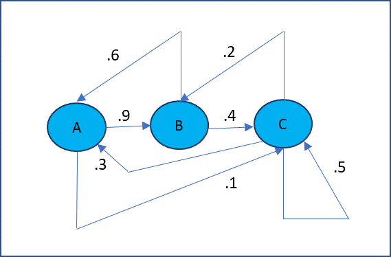
Figure 1 – Markov Chain transition diagram
The important characteristic of a Markov chain is that at any stage the next state is only dependent on the current state and not on the previous states; in this sense it is memoryless.
For our purposes here, you don’t need to know more about Markov chains, but if you are interested in learning more, click here.
Topics
Link
↑ Bayesian statistics for binomial distributions
References
Lee, P. M. (2012) Bayesian statistics an introduction. 4th Ed. Wiley
https://www.wiley.com/en-us/Bayesian+Statistics%3A+An+Introduction%2C+4th+Edition-p-9781118332573
Gelman, A., Carlin, J. B., Stern, H. S., Dunson, D. B., Vehtari, A., Rubin, D. B. (2014) Bayesian data analysis, 3rd Ed. CRC Press
https://statisticalsupportandresearch.files.wordpress.com/2017/11/bayesian_data_analysis.pdf
Marin, J-M and Robert, C. R. (2014) Bayesian essentials with R. 2nd Ed. Springer
https://www.springer.com/gp/book/9781461486862
Jordan, M. (2010) Bayesian modeling and inference. Course notes
https://www.coursehero.com/file/67562775/Stat-260-CS-294-Bayesian-Modeling-and-Inferencepdf/
Reich, B. J., Ghosh, S. K. (2019) Bayesian statistics methods. CRC Press