Cox Regression using Newton’s Method

Terminology

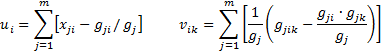
We use the following terminology for any subject s, for any j = 1, …, m and for any i and k = 1, …, r

We also assume that d_j = 1 for all times t_j and define g_j(X) = g_s(X) where s is the unique subject that dies at time t_j.

Newton’s Method

Property 1 (Newton-Raphson): We can estimate the r × 1 coefficient matrix B = [b_i] as B_p for some large enough p, where B₀ consists of all zeros (initial guess) and for all p

where  = [v_ik] is the r × r (information) matrix and U_p = [u_i] is the r × 1 (score) matrix where we use the coefficients b₁, …, b_r in B_p in calculating u_i and v_ik.

In addition, I_p is the covariance matrix for B_p at each step p in the iteration.

Example of Newton’s Method

Example 1: Find the standard error of the correlation coefficients calculated in Example 1 of Cox Regression using Solver and test whether each coefficient is significantly different from zero.

Instead of going through all the steps of Newton’s Method, we will show how to use the fact that  is the covariance matrix for B to address Example 1.

Figure 1 – Calculation of Coefficient Covariance Matrix

Key formulas from Figure 1 are shown in Figure 2 (with references to Figure 3 of Cox Regression using Solver).

Cells	Entity	Formula
Q4	g1	=L4+Q5
R4	g11	=I4*L4+R5
S4	g12	=J4*L4+S5
T4	u11	=IF(H4=1,I4-R4/Q4,0)
U4	u12	=IF(H4=1,J4-S4/Q4,0)
V4	g111	=I4*I4*L4+V5
W4	g112	=I4*J4*L4+W5
X4	g122	=J4*J4*L4+X5
Y4	v111	=IF(H4=1,(V4-R4*R4/Q4)/Q4,0)
Z4	v112	=IF(H4=1,(W4-R4*S4/Q4)/Q4,0)
AA4	v122	=IF(H4=1,(X4-S4*S4/Q4)/Q4,0)
T22	u1	=SUM(T4:T21)
U22	u2	=SUM(U4:U21)
Y22	v11	=SUM(Y4:Y21)
Z22	v12	=SUM(Z4:Z21)
AA22	v22	=SUM(AA4:AA21)
AC4	v11	=Y22
AC5	v21	=Z22
AD4	v12	=Z22
AD5	v22	=AA22
AC8:AD9	cov matrix	=MINVERSE(AC4:AD5)
AC12	u1	=T22
AC13	u2	=U22

Figure 2 – Key formulas from Figure 1

Observations

First, we note that when Solver (or Newton’s Method) converges to a solution the value of the U vector will be close to a zero vector. Based on the values in B and the covariance matrix, we can create the output shown in Figure 3.

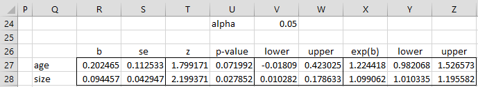
Figure 3 – Cox Regression output

We see from Figure 3 that the Age coefficient is not significantly different from 0, but the Size coefficient is significantly from zero. Except for the values of the regression coefficients, the estimates given in Figure 3 are based on having a large enough sample so that the regression coefficients follow a normal distribution.

The formulas for the Age row of Figure 3 are shown in Figure 4 (with references to Figure 3 of Cox Regression using Solver and Figure 1 above). The Size entries are similar.

Cells	Entity	Formula
R27	coefficient b1	=O4
S27	s.e.	=SQRT(AC8)
T27	z	=R27/S27
U27	p-value	=2*(1-NORM.S.DIST(T27,TRUE))
V27	1-α CI lower	=R27-S27*NORM.S.INV(1-V24/2)
W27	1-α CI upper	=R27+S27*NORM.S.INV(1-V24/2)
X27	exp(b)	=EXP(R27)
Y27	1-α CI low	=EXP(V27)
Z27	1-α CI upper	=EXP(W27)

Figure 4 – Key formulas from Figure 3

Confidence intervals for both the regression coefficients (range V27:W28) as well as the exponential of the regression coefficients (range Y27:Z28) are shown in Figure 3. Note too that sometimes the Wald value of the coefficients is calculated (as for logistic regression); these are equal to z². In this case, the p-values can be calculated using the chi-square distribution; e.g. the p-value for b₁ can be calculated using the formula =CHISQ.DIST.RT(T27^2,1), yielding the same value shown in cell U27.

Increased Risk

Example 2: How much does the risk of cancer increase for a tumor of size 10 compared with one of size 8, based on the model in Example 1 (for subjects of the same age)?

Since we don’t know the age of the subject under consideration, we will simply compare X₁ = (age, 8) with X₂ = (age, 10) for any value of age.  Since

we know that

Thus the hazard ratio (i.e. relative risk) is

Observation: The same line of reasoning shows that for any regression coefficient b_i, e^b_i is the relative increase in risk based on one unit of increase of the i^th covariate assuming the values of all other covariates are held constant. An equivalent interpretation is that b_i is the natural log of the hazard ratio when the value of x_i is increased by one unit.

Example 3: How much does the risk of cancer increase for a 70-year old with a tumor of size 5 (profile 2) compared with a 65-year old with a tumor of size 10 (profile 1), based on the model in Example 1? Also, give the 95% confidence interval for this increase.

We see that a subject with profile 2 is 71.6% more at risk of dying of cancer than a subject with profile 1. To get the 95% confidence interval, first, we need to calculate the standard error. To do this, we calculate the variance of the nature log and use the fact that var(x+y) = var(x) + var(y) + 2cov(xy). Thus, using the covariance matrix of range AC8:AD9 of Figure 1

= 25(.012664 + .001844 – 2 · .002877) = .2188

Thus the standard error = .4678. The 95% confidence interval for the natural log of the hazard ratio is therefore

Taking the exponential of this interval, we see that the 95% confidence interval for the hazard ratio is (.686, 4.29).

References

NCSS (2015) Cox regression
https://www.ncss.com/wp-content/themes/ncss/pdf/Procedures/NCSS/Cox_Regression.pdf
Collett, D. (2003) Modelling survival data in medical research. 2nd ed. Chapman & Hall/CRC
Zhang, D. (2011) Modeling survival data with Cox regression models
https://www.scribd.com/document/396594178
Wikipedia (2015) Proportional hazards model
https://en.wikipedia.org/wiki/Proportional_hazards_model
Grund, B., Yang, L. (2015) Hazard regression
https://edoc.hu-berlin.de/server/api/core/bitstreams/595cb9b6-0c1a-4121-8a83-8a194f19b3ae/content
Hello, Professor, I ask you a question, which I don’t know if it really makes sense.
Is it possible to express the calculation of the columns from “Q” (column “G”) to “AA” (column “V22”) of figure 1 in example 1 in matrix form, in order to speed up the calculation of the coefficients, of the covenrgence matrix and of the covariance matrix?
I greet you cordially, Roberto
Hello Roberto,
Perhaps, but when I created this spreadsheet such an approach didn’t occur to me, and I haven’t thought about it since then.
Sorry that I don’t have a more helpful answer for you.
Charles
Hello Charles,
I´ve got a question concerning Example 3. If you write below Fig.3 that “We see from Figure 3 that the Age coefficient is not significantly different from 0”, shouldn´t we set b(age) to zero?
Hello Jiří,
No. The coefficient is whatever value is calculated. If you set the significance level to alpha = .10 (instead of alpha = .05), then the coefficient would be significantly different from zero.
Dear Charles,
You state on this website
“To do this, we first calculate the variance of the nature log and use the fact that var(x+y) = var(x) + var(y) + 2cov(xy). Thus, using the covariance matrix of range AC8:AD9 of Figure 1”
The outcome of the sum then presented according to my calculator should be .21885 in stead of .2821 Then the outcome of the s.e being .4678 also makes sense again. As .4678^2 equals .21885
Hi Tim,
Yes, you are correct. I don’t know where the .2821 value came from since the spreadsheet contains the correct value.
In any case, thank you very much for catching this error. I have now corrected it on the website.
Prof, can Cox Regression be appropriate for categorical (0,1) predictors? When comparing two cases/samples – basically the differences are the predictors.
Hi Dominic,
Yes, categorical variables can be used.
Hi Charles,
You’ve got cell Q4 = L4*Q5. Should this be Q4 = L4 + Q5?
Thanks,
Brendan
Hi Brendon,
Thanks for catching this mistake and improving the accuracy of the website. I have now corrected the error on the webpage.