Markov Chains Limiting Probabilities

Limiting Probabilities

Definition 1: Suppose that the limit on the left side of the following equation exists for all r, s in S and suppose further that

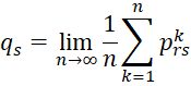
for any r and u in S. Then we can define the limiting probability at s to be

Property 1: The limiting probabilities p_s are the unique solution to the equations (for all s in S)

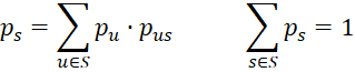
Proof: By Property 1 of Markov Chains Basic Concepts

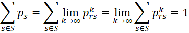
Finally, we need to show that the system of linear equations has a unique solution. Let q_s for all s in S be a solution to the equations and let Q be the n × 1 vector Q = [q_s], where n = the number of states in S, and let P be the n × n matrix P = [p_rs]. Since

we see that Q = QP. It then follows that QP = QP² and hence Q = QP². In a similar fashion it follows that Q = QP^k. This means that

From this and the assumption that

it follows that

This completes the proof.

Property 2: For any states r and s, the following limit always exists

Proof: In general, for any sequence a₁, a₂, …, the Cesàro limit

exists and is equal to the limit of a_n as n → ∞ if this ordinary limit exists.

Periodic chains

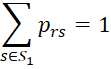
Definition 2: A Markov chain is periodic if there is a non-empty partition of S = S₁ ⋃ S₂ ⋃ … ⋃ S_m with m > 1 and S_i ⋂ S_j = ∅ for all i ≠ j such that if r ∈ S_i with i < m then

(i.e. p_rs = 0 for any s not in S_i+1) and for any r ∈ S_m then

(i.e. p_rs = 0 for any s not in S₁).

For example, S = {1, 2} where p₁₂ = p₂₁ = 1 (and so p₁₁ = p₂₂ = 0) is a trivial example of a periodic Markov chain.

Stationary chains

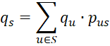
Definition 3: A probability distribution f(s) = q_s on S is an equilibrium (aka stationary) distribution of a Markov chain if

The first set of equations are called the equilibrium equations and the last equation is called the normalizing equation. If S has n elements, then these equations can be re-expressed as n-1 equation in n-1 unknowns.

Let Q be the n × 1 vector Q =[q_s] and let P be the n × n matrix P = [p_rs]. Then, as we saw in the proof of Property 3, the equilibrium equations can be expressed as Q = QP.

The reason for calling q_s a stationary distribution is explained in the following property.

Property 3: If q_s is an equilibrium distribution and P(x₀ = s) = q_s for all s, then for all i and all s, P(x_i = s) = q_s.

Proof: The proof is by induction on i. The case i = 0 is obvious. Assume the property for i. Now

Observation: If the limiting probabilities exist for all states s, then by Property 1, f(s) = p_s is the unique equilibrium distribution. Unfortunately, these limiting probabilities don’t always exist; e.g. if the set of states is periodic.

Definition 4: A non-empty set of states C is closed provided there is no transition out of C, i.e. for all r in C and s not in C, p_rs = 0.

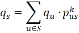
Property 4: A (finite-state) Markov chain x₀, x₁, … which does not contain two or more disjoint closed sets has a unique equilibrium distribution q_s such that for any states s

where q_s is independent of the starting state r.

Furthermore, if the Markov chain is not periodic, then the p_s exist, and so q_s = p_s.

Observations

Note that the Markov chain in Example 2 of Markov Chain Examples is not periodic and does not contain two or more disjoint closed sets. Thus the p_s exist and satisfy the equilibrium equations of Definition 3. This explains why the  arising from high powers of P^k (corresponding to the limit of the p^k_rs as k → ∞) were the same as the solutions to the simultaneous linear equations (as in Definition 3).

Note too that if the Markov chain has more than one disjoint closed sets, then each such closed set would satisfy Property 4.

References

Fewster, R. (2014) Markov chains
https://www.stat.auckland.ac.nz/~fewster/325/notes/ch8.pdf

Pishro-Nik, H. (2014) Discrete-time Markov chains
https://www.probabilitycourse.com/chapter11/11_2_1_introduction.php

Norris, J. (2004) Discrete-time Markov chains
https://www.statslab.cam.ac.uk/~james/Markov/

Lalley, S. (2016) Markov chains
https://galton.uchicago.edu/~lalley/Courses/312/MarkovChains.pdf

Konstantopoulos, T. (2009) Markov chains and random walks
https://www2.math.uu.se/~takis/L/McRw/mcrw.pdf

Wikipedia (2025) Cesàro summation
https://en.wikipedia.org/wiki/Ces%C3%A0ro_summation