Markov Chain Examples

Introduction

We illustrate some of the concepts from Markov Chains Basic Concepts via some examples in Excel.

Example 1

What is the probability that it will take at most 10 throws of a single die before all six outcomes occur?

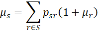
Let S = {0,1,2,3,4,5,6} and x_i = the number of different outcomes that have occurred by time i. Clearly, {x₀, x₁, ….} is an absorbing Markov chain where 6 is an absorbing state and x₀ = 0. We start by observing that

Using this information, we can represent the transition probability matrix P as shown in Figure 1.

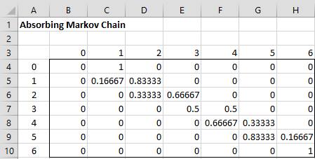
Figure 1 – Transition Probability Matrix

Now, let z be a random variable that z or fewer throws of a single die before all six outcomes occur.

Since 6 is an absorbing state for any k, it follows that

Thus, the probability that it will take at most 10 throws of a single die before all six outcomes occur is p¹⁰₀₆. We need to calculate the 10-step transition probability matrix as shown in Figure 2.

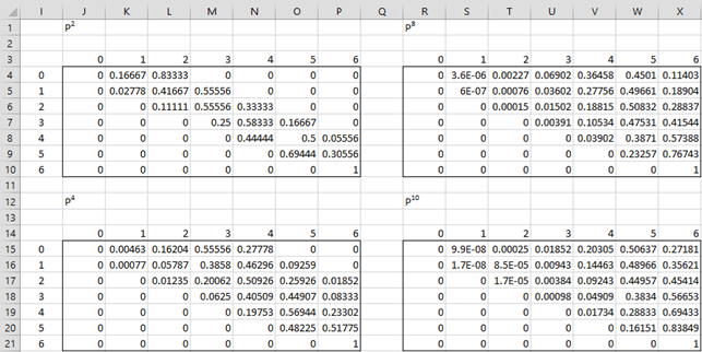
Figure 2 – 10-step Transition Probability Matrix

P² is calculated using the array formula =MMULT(B4:H10,B4:H10), P⁴ is calculated by the array formula =MMULT(J4:P10,J4:P10), P⁸ is calculated by =MMULT(J15:P21,J15:P21) and P¹⁰ is calculated by =MMULT(R4:X10,J4:P10).

Thus, the probability that it will take at most 10 throws of a single die before all six outcomes occur is p¹⁰₀₆ = .27181 (cell X15).

Actually, the P¹⁰ matrix in range R15:X21 of Figure 2 can be calculated using the Real Statistics array formula =MPOWER(B4:H10,10). Note that we can calculate the value p⁹₀₆ = .1890 by using the formula =INDEX(MPOWER(B4:H10,10),1,7). Thus, the probability that it will take exactly 10 throws of a single die before all six outcomes occur is .27181 – .18904 = .08277.

Example 2

A die is repeatedly rolled. Bob wins a roll when 3, 4, 5 or 6 comes up and Jim wins a roll when 1 or 2 comes up. Bob wins the game if he wins 3 rolls in a row and Jim wins if he wins two rolls in a row. Determine the probability that Bob wins within 20 rolls. Determine the probability that Bob will win.

The first problem is similar to that of Example 1. The set of states S = {0, 1, 2, 3, a, b} where

0 = initial state

1 = Bob has won the last roll (but not the previous roll)

2 = Bob has won the last two rolls

3 = Bob has won three rolls in a row (absorbing state)

a = Jim has won the last roll

b = Jim has won two rolls in a row (absorbing state)

Thus

p₀₁ = p₁₂ = p₂₃ = p_a1 = 2/3

p_0a = p_1a = p_2a = p_ab = 1/3

p₃₃ = p_bb = 1

and all other one-state transition probabilities are zero.

The one-state transition probability matrix is shown in Figure 3.

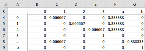
Figure 3 – Transition Probability Matrix

Result

We now calculate P¹⁰, P²⁰, P³⁰ and P⁴⁰ using the MPOWER function, as shown in Figure 4.

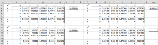
Figure 4 – Iteration to a Solution

From cell M20, we see that the probability that Bob wins within 20 rolls of the die is 60.64%. The probability that Jim wins within 20 rolls is 37.24% (cell O4). The probability that someone wins within 20 rolls is therefore 60.64% + 37.24% = 99.55% (cellQ4).

Note that as we increase the number of rolls, two things happen. First, the probability that someone wins approaches 100%. E.g. after 40 rolls, this probability has already reached 100% (cell AA12), at least to 5 decimal places. Second, successive values of P^k don’t change much (convergence), as can be seen by comparing P³⁰ with P⁴⁰.

From cell W12, we see that the probability that Bob wins is 62.75%. The probability that Jim wins is 37.25%.

Alternative Approach

We now show another way of calculating the probability that Bob wins. Let q_s be the probability that Bob wins starting with state s. By the law of conditional probability it follows that

Thus

where q₃ = 1  and q_b = 0. We now solve these equations.

and so q₁ = 12/17. Thus

It now follows that

which is the same answer we got previously.

Example 3

Find the expected number of rolls before someone wins the game described in Example 2.

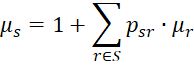
Once again we need a set of simultaneous equations. Let μ_s be the expected number of rolls until someone wins starting with state s. By the law of conditional expectations, it follows that

Since

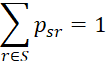
we conclude that

But note that p₀₁ = p₁₂ = p₂₃ = p_ab = 2/3 and p_0a = p_1a = p_2a = p_ab = 1/3. All other p_sr = 0. Hence

where μ₃ = μ_a = 0. We now solve the four equations in four unknowns. Actually, without the first equation, we have three equations in three unknowns. We start with

which is equivalent to

which means that

and so

Finally, we see that

We now find the other expected values as follows

Examples Workbook

Click here to download the Excel workbook with the examples described on this webpage.

References

Fewster, R. (2014) Markov chains
https://www.stat.auckland.ac.nz/~fewster/325/notes/ch8.pdf

Pishro-Nik, H. (2014) Discrete-time Markov chains
https://www.probabilitycourse.com/chapter11/11_2_1_introduction.php

Norris, J. (2004) Discrete-time Markov chains
https://www.statslab.cam.ac.uk/~james/Markov/

Lalley, S. (2016) Markov chains
https://galton.uchicago.edu/~lalley/Courses/312/MarkovChains.pdf

Konstantopoulos, T. (2009) Markov chains and random walks
https://www2.math.uu.se/~takis/L/McRw/mcrw.pdf