Basic Concepts
We can compare the observed values yi with the values μi predicted by a Poisson regression model. In addition, we can calculate standard errors for these predictions along with confidence intervals. The standard error and 1 – α confidence interval are given by the formulas
![]()
where zcrit = NORM.S.INV(1-α/2), and S and Xi are as described in Poisson Regression using Solver.
Example
The predicted values, as well as the standard error of the prediction and 95% confidence intervals for the 15 observations in Example 1 of Poisson Regression using Solver, are shown in Figure 1.
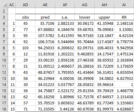
Figure 1 – Predictions corresponding to observations
Here, columns AD and AE are copied from columns J of Figure 2 and Q of Figure 3 of Poisson Regression using Solver. The array formula used to calculate the standard error of the prediction for the first observation (cell AF4) is
=Q4*SQRT(MMULT(MMULT(F4:I4,$F$23:$I$26), TRANSPOSE(F4:I4)))
Predictions for Unobserved Values
If you want to predict a value that was not observed, then you can use the same formula, where you explicitly supply values for Psych, Cig, and Pop. The predicted number of tumors in a population of 10,000 people who have psychological profile A and smoke 1.25 packs of cigarettes a day is given in row 4 of Figure 2.
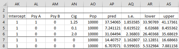
Figure 2 – Predictions
Cell AP4 contains the formula
=AO4*EXP(SUMPRODUCT(AK4:AN4,F$20:I$20))
Cell AQ4 contains the array formula
=AP4*SQRT(MMULT(MMULT(AK4:AN4,$F$23:$I$26),TRANSPOSE(AK4:AN4)))
Finally, cell AR4 contains the formula =AP4-AQ4*N$9 and cell AS4 contains the formula =AP4+AQ4*N$9 where N9 refers to a cell in Figure 2 of Poisson Regression using Solver.
Rate ratio
Column AI of Figure 1 specifies the rate ratio for the given reference observation, which for Example 1 is chosen to be observation 11, the population of people who smoke no cigarettes and have psychological profile C. The rate ratio for observation 1 (no cigarettes, profile A) is 2.148, as shown in cell AI4 (using the formula =P4/P$14 with reference to cells in Figure 3 of Poisson Regression using Solver). Thus, we can conclude that for two populations of the same size, the first consisting of non-smokers with profile A and the second non-smokers with profile C, the first population will have 2.148 times the number of tumors.
We can also see this in Figure 2 since for a population of size 10,000, the first population is expected to have 14.4 tumors (cell AP7), while the second is expected to have 6.7 tumors (cell AP8). The ratio of these two values is 2.148.
Worksheet Functions
Real Statistics Functions: The Real Statistics Resource Pack provides the following array function to assist in making predictions from a Poisson regression model with coefficients in the k+1 × 1 array Rc.
PoissonPredC(Rx0, Rc, Rt0): returns a column array containing the predicted values corresponding to the X vector in each of n rows in Rx0, and frequency value in the same row of Rt0.
The output is an n × 1 array (or numeric value if n = 1). Rx0 should have k columns. If Rt0 is omitted, it defaults to a column array of all ones with n rows. If Rt0 is not omitted, then it must either be a column array with n rows or a numeric value. When Rt0 is a numeric value, it is treated as a column array with n rows, all of whose values are equal to the specified numeric value.
The following array function is also supported, where Rv is the k+1 × k+1 covariance matrix.
PoissonPredCC(Rx0, Rc, Rv, lab, Rt0, alpha): returns an array with 4 columns, where each row contains the predicted values corresponding to the X vector in the corresponding row in Rx0 and frequency value in the same row of Rt0 (as for PoissonPredC), plus the standard error and the endpoints of the 1 – alpha confidence interval; if lab = TRUE (default FALSE), then an extra row is appended to the output containing labels; alpha is the significance level (default .05).
The Real Statistics Resource Pack also provides the following array function. This function produces predictions for a Poisson regression model based on an X array Rx (with k columns), Y array Ry, and frequency array Rt.
PoissonPred(Rx0, Rx, Ry, lab, Rt0, Rt, alpha, iter, guess): equivalent to PoissonPredCC(Rx0, Rc, Rv, lab, Rt0, alpha) where Rc is the coefficient array for the regression model, and Rv is the covariance matrix.
Examples
For Example 1 of Poisson Regression using Solver, you could use the array formula =PoissonPredC(AL7:AN7,$Q$23:$Q$26,AO7) to obtain the predicted value shown in cell AP7 of Figure 2. To obtain the predictions shown in range AP4:AP6 you could use the array formula =PoissonPredC(AL4:AN6,$Q$23:$Q$26,AO4:AO6).
To obtain the results shown in range AP3:AS6, you could use the following array formula
=PoissonPredCC(AL4:AN6,$Q$23:$Q$26,$F$23:$I$26, TRUE,AO4:AO6)
You can replace the AO4:AO6 argument in this formula with AO4 or 10000. Alternatively, you can use
=PoissonPred(AL4:AN6,$G$4:$I$18,$J$4:$J$18,TRUE, AO4,$K$4:$K$18)
Probability
What is the probability that 40 people out of 1,000 people who smoke 1.25 packs of cigarettes a day and have psychological profile A develop a tumor? What is the probability that more than 40 such people develop a tumor?
From the first row of Figure 2, we see that the mean number of tumors out of a population of 10,000 for people with the specified profile, 37.54 develop a tumor. Since the data follows a Poisson distribution, the probability that 40 people develop a tumor is
POISSON.DIST(40, 37.54,FALSE) = .058174
and the probability that more than 40 people develop a tumor is
1-POISSON.DIST(40, 37.54,TRUE) = .307206
Worksheet Functions
Real Statistics Functions: The Real Statistics Resource Pack provides the following array function.
PoissonProb(Rx0, Rc, Ry0, Rt0): returns a column array containing the probability values corresponding to the X vector in each of n rows in Rx0, the y count values in the same row of Ry0, and frequency value in the same row of Rt0 based on the Poisson regression model with coefficients in the k+1 × 1 array Rc.
The output is an n × 1 array (or numeric value if n = 1). Rx0 should have k columns. If Ry0 is omitted, it defaults to a column array of all zeros with n rows. If Rt0 is omitted, it defaults to a column array of all ones with n rows. When Ry0 or Rt0 is not omitted, then it must either be a column array with n rows or a numeric value. When Ry0 or Rt0 is a numeric value, it is treated as a column array with n rows, all of whose values are equal to the specified numeric value.
Example
We consider two of the profiles from Figure 2, namely those corresponding to rows 6 and 7. Since the mean predicted value for the first of these profiles (Psy C + 2 packs of cigarettes a day) is 31.04494, we see that the probability of 30 tumors out of 10,000 subjects is .071354, as shown in cell G6 of Figure 3. This probability could be obtained using the formula =POISSON.DIST(30,31.04494,FALSE).
For the second profile (Psy A + 0 packs per day), we see from Figure 2 that the mean number of tumors out of a population of 10,000 is 14.40757. Thus, the mean number tumors for a population of 1,000 is one-tenth of this value, namely 1.440757, as shown in range E9:E14. E.g. the probability of 1 tumor out of a population of 1,000 is .341097 (cell G10 of Figure 3), as calculated by the formula =POISSON.DIST(1,1.440757,FALSE).

Figure 3 – Probabilities
We can also obtain the probabilities in range G3:G14 of Figure 3 without using the mean predicted values from Figure 2, by using the array formula
=PoissonProb(A3:C14,J3:J6,F3:F14,D3:D14)
Examples Workbook
Click here to download the Excel workbook with the examples described on this webpage.
Links
References
Hintze, J. L. (2007) Poisson regression. NCSS
https://www.ncss.com/wp-content/themes/ncss/pdf/Procedures/NCSS/Poisson_Regression.pdf
Nussbaum, E. M., Elsadat, S., Khago, A. H. (2007) Best practices in evaluating count data, Chapter 21: Poisson regression.
http://www.academia.edu/438746
Penn State (2017) Poisson regression. STAT 504: Analysis of discrete data.
https://online.stat.psu.edu/stat504/Lesson09