Second Order Differential Equations

Basic Concepts

We now describe how to solve second order differential equations of the following form numerically.

y′′ = f(x, y, y′)          y(x₀) = y₀          y′(x₀) = y₁

These sort of equations can be expressed as simultaneous differential equations as follows where z = y’:

y′ = z          y(x₀) = y₀

z′ = f(x, y, z)          z(x₀) = y₁

We can then use the methods for simultaneous differential equations to solve second order differential equations. In particular, we can use the following approaches.

Euler’s method

k₁ = hf(x_i, y_i, z_i)           m₁ = hz_i

y_i+1 = y_i + k₁          z_i+1 = z_i + m₁

Runge-Kutta (RK2)

k₁ = hf(x_i, y_i, z_i)           m₁ = hz_i

k₂ = hf(x_i+h/(2b), y_i+k₁/(2b), z_i+m₁/(2b))           m₂ = h(z_i+m₁/(2b))

y_i+1 = y_i + [(1-b)k₁ + bk₂]       z_i+1 = z_i + [(1-b)m₁ + bm₂]

Runge-Kutta (RK4)

k₁ = hf(x_i, y_i, z_i)           m₁ = hz_i

k₂ = hf(x_i+h/2, y_i+k₁/2, z_i+m₁/2)           m₂ = h(z_i+m₁/2)

k₃ = hf(x_i+h/2, y_i+k₂/2, z_i+m₂/2)           m₃ = h(z_i+m₂/2)

k₄ = hf(x_i+h, y_i+k₃, z_i+m₃)           m₄ = h(z_i+m₃)

y_i+1 = y_i + (k₁+2k₂+2k₃+k₄)/6              z_i+1 = z_i + (m₁+2m₂+2m₃+m₄)/6

Worksheet Function

The Real Statistics Resource Pack provides the following worksheet function that uses Real Statistics lambda capabilities.

DiffEq2(xx, R1, x₀, y₀, y₁, h, ttype, b, Rx, Ry, Rz) = the solution to the differential equations y′′ = f(x,y,y′) at the specified x value xx based on the initial values of y(x₀) = y₀ and y′(x₀) = y₁

Here R1 contains the expression for f(x,y,z) using the lambda approach described in Differential Equations Support. h is a small positive numeric value as described above. ttype takes the values “ef” for the Euler forward method, “tr” for Heun’s method, “rk” or “rk2” for the Runge-Kutta order 2 method (default) and “rk4” for the Runge-Kutta order 4 method. If ttype = “rk” or “rk4” then b is as defined in Other Methods for Solving Differential Equations.

Rx is the cell address in R1 that points to the x value, Ry is the cell address in R2 that points to the y value, and Rz is the cell address in R2 that points to the z value. If Rx is omitted then x is the first relative cell address in R1 (without a $). If Ry is omitted then y is the second relative cell address in R1. Finally, if Rz is omitted then z is the third relative cell address in R1,

If xx–x₀ is not evenly divisible by h, this function uses linear interpolation.

Examples

Example 1: Solve the differential equation

y′′ + 4y = sin(3x)          y(0) = 1          y′(0) = 2

It turns out that the analytic solution is

y = cos(2x) + 10/13 ⋅ sin(2x) – 1/5 ⋅ sin(3x)

We use Euler’s method with h = .1, as shown in Figure 1 (only the first half of the rows are shown in the figure).

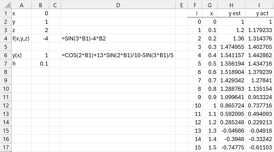
Figure 1 – Second-order differential equation

Here, cell H2 contains the formula =DiffEq2(G2,B$4,B$1,B$2,B$3,B$7,”ef”) and cell I2 contains the formula =EVALS(B$6,G2). A chart of the solution is shown in Figure 2.

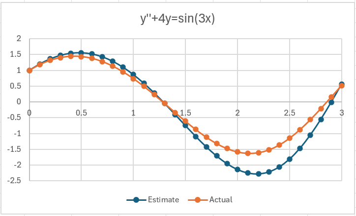
Figure 2 – Chart of the solution

As you can see, the estimate is reasonably close to the actual solution. Using the RK2 or RK4 method provides much better results.

Example 2: Solve the differential equation

y′′ + 5y′ + 6y = 10 sin x          y(0) = 0          y′(0) = 5

It turns out that the analytic solution is

y = -6 exp(-3x) + 7 exp(-2x) + sin x – cos x

This time we use the RK2 method with h = .1, as shown in Figure 3 (only the first few rows of the output are shown in the figure).

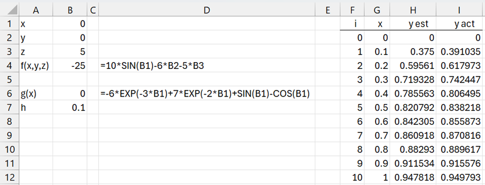
Figure 3 – Second-order differential equation

The corresponding chart is shown in Figure 4.

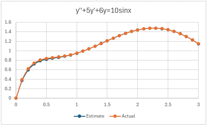
Figure 4 – Second-order differential equation chart

As you can see, the estimate is quite close to the actual solution.

Examples Workbook

Click here to download the Excel workbook with the examples described on this webpage.

References

Strang, G., Herman, E., Seeburger, P. (2025) Introduction to differential equations
https://math.libretexts.org/Courses/Monroe_Community_College/MTH_211_Calculus_II/Chapter_8%3A_Introduction_to_Differential_Equations/8.1%3A_Basics_of_Differential_Equations

Atkinson, K., Han, W., Stewart, D. (2009) Numerical solutions to ordinary differential equations. Wiley-Interscience
https://homepage.math.uiowa.edu/~atkinson/papers/NAODE_Book.pdf

Hossain, J., Alam, S., Hossain, B. (2017) A study on numerical solutions of second order initial value problems (IVP) for ordinary differential equations with fourth order and Butcher’s fifth order Runge-Kutta methods
http://article.sapub.org/10.5923.j.ajcam.20170705.02.html

Wikipedia (2025) Numerical methods for ordinary differential equations
https://en.wikipedia.org/wiki/Numerical_methods_for_ordinary_differential_equations