Objective
On this webpage we describe Real Statistics capabilities to simplify solving differential equations numerically in Excel. See Euler’s Method and More Differential Equation Methods for background information.
Worksheet Functions
The Real Statistics Resource Pack provides the following worksheet function that uses Real Statistics lambda capabilities.
DiffEq(xx, R1, x0, y0, h, ttype, iter, Rx, Ry) = the solution to the differential equation y′ = f(x, y) at the specified x value xx based on the initial value of y = y0 when x = x0.
Here R1 contains the expression for f(x, y) using the lambda approach described in Real Statistics Lambda Capabilities. h is a small positive numeric value as described above.
ttype takes the values “ef” for the Euler forward method, “eb” for the Euler backward method, “tr” for the trapezoid method, “rk” or “rk2” for the Runge-Kutta (RK2) method (default “rk”), or “rk4” for the Runge-Kutta (RK4) method. If ttype = “eb” or “tr” then iter = the number of iterations used (default 2). If ttype = “rk” or “rk2” then iter = the b parameter (default .5) defined in More Numerical Differential Equation Methods.
Rx is the cell address in R1 that points to the x value and Ry is the cell address in R2 that points to the y value. If Rx is omitted then x is the first relative cell address in R1 (without a $). If Ry is omitted then y is the second relative cell address in R1.
Finally, if xx – x0 is not evenly divisible by h, this function uses linear interpolation to obtain a result.
Example
Example 1: Solve the differential equation
y′ = -y + 2 cos x y0 = 1
Figure 1 shows the estimated solutions for x = 2, 4, 6, 8, 10 based on various values for h and b using the Runge-Kutta method.
We created the table by inserting the formula =DiffEq($F5,$B$7,$B$2,$B$3,G$2,,G$3) in cell G5, highlighting range G5:O9, and pressing Ctrl-D and Ctrl-R.
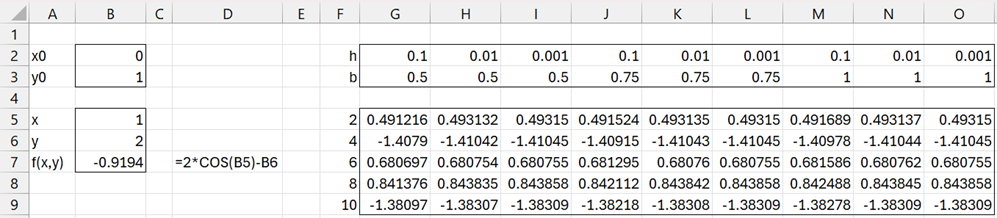
Figure 1 – Using the DiffEq function
Note that it was important that the formula in cell D7 is =2*COS(B5)-B6, i.e. the x variable (B5) precedes the y variable (B6). If you use the formula =-B6+2*COS(B5), then use need to insert the following formula in cell G5, explicitly setting values for Rx and Ry:
=DiffEq($F5,$B$7,$B$2,$B$3,G$2,,G$3,$B$5,$B$6)
Chart
Example 2: Compare the graphs of the solution to the differential equation from Example 1 of Numerical Differential Equations between x = 0 and x = 2 using numerical (using Runge-Kutta Method with h = .025 and b = 1) and analytic techniques.
The first 14 of 81 values is shown on the left side of Figure 2. We note that the plot of the estimate and actual values are so close that the curve for the estimated values is completely hidden by the actual values. Note too that, unlike in other examples on this website, the relative error increases, not decreases, although at least through x = 2 the estimates are still quite good.
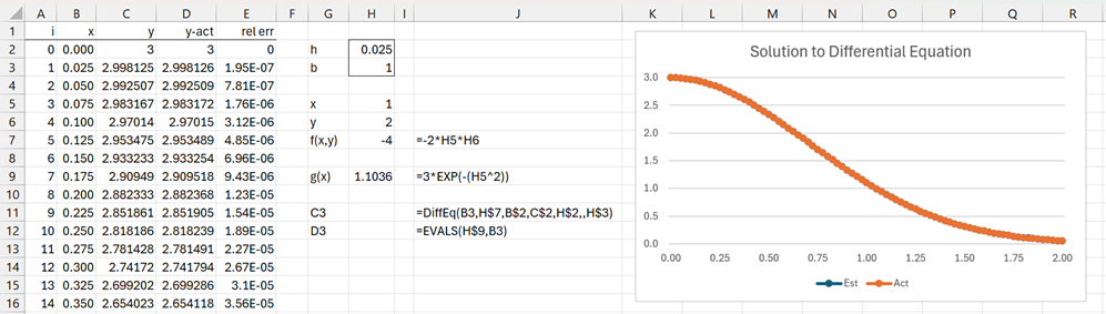
Figure 2 – Plot of Actual vs Estimate
Examples Workbook
Click here to download the Excel workbook with the examples described on this webpage.
Links
↑ Numerical differential equations
References
Strang, G., Herman, E., Seeburger, P. (2025) Introduction to differential equations
https://math.libretexts.org/Courses/Monroe_Community_College/MTH_211_Calculus_II/Chapter_8%3A_Introduction_to_Differential_Equations/8.1%3A_Basics_of_Differential_Equations
Atkinson, K., Han, W., Stewart, D. (2009) Numerical solutions to ordinary differential equations. Wiley-Interscience
https://homepage.math.uiowa.edu/~atkinson/papers/NAODE_Book.pdf
Wilson, H. J. (2025) Ordinary differential equations
https://www.ucl.ac.uk/~ucahhwi/GM01/ODE_extra.pdf
Wikipedia (2025) Numerical methods for ordinary differential equations
https://en.wikipedia.org/wiki/Numerical_methods_for_ordinary_differential_equations