Objective
We show how to use Euler’s Method to solve differential equations numerically. Even though other techniques may be more efficient, this approach provides an excellent introduction to the various techniques that are available.
Euler’s (Forward) Method
Let’s assume that
y′ = f(x, y(x)) y(x0) = y0
for all x in the interval [a, b].
Define a sequence a = x0 < x1 < … < xn = b. E.g. set h = (b–a)/n, x0 = a, and xi+1 = xi + h. Thus, xi = x0 + ih for all i. In particular, xn = a + nh = a + n(b–a)/n = b.
We also define yi = y(xi).
Since
![]()
we have
![]()
It now follows that
![]() Thus
Thus
y1 = y0 + hf(x0, y0)
y2 = y1 + hf(x1, y1)
etc.
yn = yn-1 + hf(xn-1, yn-1)
But y(b) = yn, and so this provides a recursive way to evaluate y(b).
Example of Euler’s Method
Example 1: Find y(2) for the following differential equation
y′ + 3y = 6x + 11 y(0) = 4
If we use h = .1, then the sequence of x values x0, x1, … is as shown in column B of Figure 1. The corresponding y values are shown in column C. We initialize x0 = 0 and so y0 = 4 (as shown in cell C2). We insert the formula =C2+H$2*(6*B2-3*C2+11) in cell C3, highlight range C3:C22, and press Ctrl-D to obtain the value y(2) = 7.000798, as shown in cell C22.
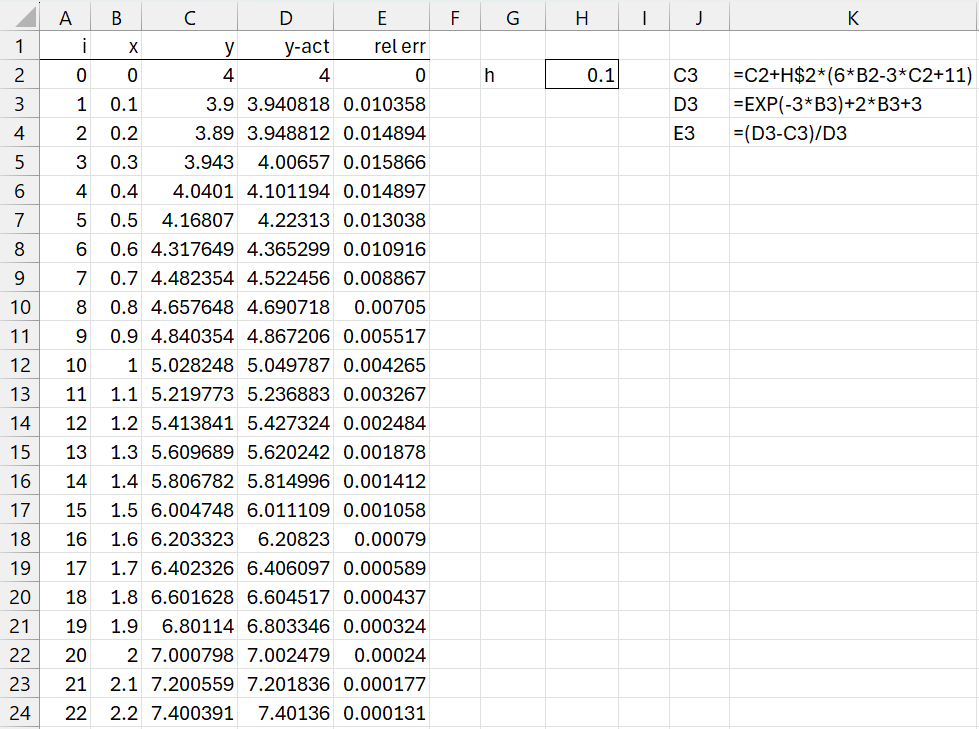
Figure 1 – Euler’s (forward) method
Actually, we can highlight as many cells in column C as we like to obtain estimates for y(x) for any x = .1n for any integer value of n that we like. We can also use interpolation to estimate values of x that are not multiples of .1.
Analytical solution
The analytic solution to the differential equation is
y = e-3x + 2x + 3
We can check the initial value as follows
y(0) = e-3(0) + 2(0) + 3 = 1+ 0 + 3 = 4
We can check that this is a solution to our differential equation as follows
y′ + 3y = (-3x + 2) + 3(e-3x + 2x + 3)
= -3x + 2 + 3e-3x + 6x + 9 = 6x + 11
If we plug in the values of e-3x + 2x + 3 for each value of x in column B of Figure 1, we get the corresponding y values as shown in column D. From this, we can calculate how good the estimates we obtained from Euler’s method, as shown in column E.
We see that the actual value for y(2) = 7.002479 (cell D22), a relative error of 0.024% (cell E22).
Observations
Often, the further away the x = b is from the initial value, the better the estimate. E.g. for Example 1, y(3) = 9.000123 whereas the Euler estimate is 9.000023, a relative error of only 0.00112%. Also, the smaller the value of h, the longer it takes the algorithm to calculate a solution, but the more accurate the solution. E.g. with h = .01, y(2) = 7.002261, a relative error of 0.000311%, but instead of 20 steps, it now takes 200 steps to find the answer. In fact, with h = .00001, the estimate at x = 2 matches the actual result to 6 decimal places.
If the actual solution to the differential equation is known then you can calculate its error and relative error, but if the actual solution is not known, then you can use Richardson’s estimate of the error, namely
y(x) – yh(x) ≈ yh(x) – y2h(x)
Using Real Statistics Lambda Capability
We can also perform the analysis using Real Statistics’ lambda capabilities, as shown in Figure 2 (only the first few lines are displayed). The results, of course, are the same as shown in Figure 1.
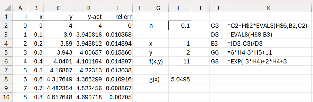
Figure 2 – Euler’s method using EVALS
Examples Workbook
Click here to download the Excel workbook with the examples described on this webpage.
Links
↑ Numerical differential equations
References
Strang, G., Herman, E., Seeburger, P. (2025) Introduction to differential equations
https://math.libretexts.org/Courses/Monroe_Community_College/MTH_211_Calculus_II/Chapter_8%3A_Introduction_to_Differential_Equations/8.1%3A_Basics_of_Differential_Equations
Atkinson, K., Han, W., Stewart, D. (2009) Numerical solutions to ordinary differential equations. Wiley-Interscience
https://homepage.math.uiowa.edu/~atkinson/papers/NAODE_Book.pdf
Wilson, H. J. (2025) Ordinary differential equations
https://www.ucl.ac.uk/~ucahhwi/GM01/ODE_extra.pdf
Wikipedia (2025) Numerical methods for ordinary differential equations
https://en.wikipedia.org/wiki/Numerical_methods_for_ordinary_differential_equations