Data Analysis Tool
We can use Real Statistics’ Solving Differential Equations data analysis tool to solve first and second order differential equations.
First Order Example
Example 1: Solve the differential equation for values of x in the interval [1,3]
y’=x*y-ln(x+1)^y-2*x+1+exp(x)/2 y(1) = 2
Press Ctrl-m and choose Solving Differential Equations from the Misc tab. Next, fill in the dialog box that appears as shown in Figure 1.
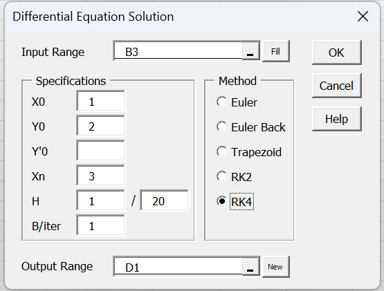
Figure 1 – Differential Equations dialog box
After clicking on the OK button, the output in Figure 2 appears (only value of x up to 1.8 are displayed).
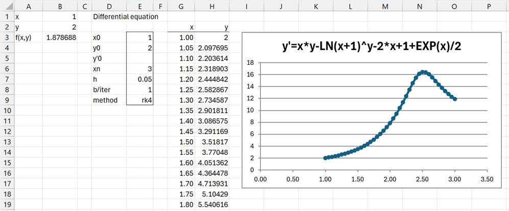
Figure 2 – First order differential equation solution
Dialog Box
Use of decimal numbers
In Figure 1, we specified that the H field contains the values 1/20 = .05. You could also use .05 and leave the second field blank (alternatively, you could use .05/1). The reason for using a fraction is that not everyone uses a period as the decimal symbol. When a comma is used as the decimal symbol, 0,05 is not an acceptable entry, and so such users can employ the fraction 1/20.
The situation is similar for all the other fields. E.g. if you use a period as the decimal symbol, you could insert the value such as 3.5 in the Y0 field. If, instead, you use a comma as the decimal symbol, you should use a whole number such as 3 instead. After pressing the OK button on the dialog box, you can then change the value in the output to the desired value, including decimal values using a comma. For this example, this would mean changing the value in cell E4 of Figure 2.
Other changes you can make
You can also change the Method in cell E9 to any of the other valid methods (“ef”, “eb”, “tr”, “rk2”, or “rk4”). If you use “eb” or “tr” you can change the number of iterations (cell E8). Similarly, if you use the “rk2” method you can change the b values. Users of Excel that employ a comma as the decimal symbol can change the value in cell E8 from 1 to 0,5. Alternatively, they can enter “tr” in cell E9 and 1 in cell E8 (since this results in Heun’s method in either case).
After any of these changes, the values displayed and the chart will change automatically although some modifications to the chart axes might be required.
You can also change the formula in cell B3, although in this case, you will need to change the chart title.
You can also change the values of x0, xn, and h (in cells E3, E6 and E7 of Figure 2), except that you can’t change the value of (xn–x0)/h. E.g. if x0 = 1, xn = 3, and h = .1, you can change x0 to 0.5 (or 0,5 when comma is the decimal symbol), but in this case the output will change to values between x = 0.5 and x = 2.5 in increments of h = .1. Similarly, if x0 = 1, xn = 3, and h = .1, and you change h to .05 (or 0,05), then the output will change to values between x = 0 and x = 1.5 in increments of h = .05.
Y′0 field
Finally, note that since Example 1 specifies a first order differential equation, you need to leave the Y′0 field blank in the dialog box. Any changes to y′0 in the output (cell E5 of Figure 2) will be ignored.
Second Order Example
Example 2: Repeat Example 1 of Second Order Differential Equations using the Differential Equations data analysis tool. This time we will use the RK2 method with h = .1
Press Ctrl-m and choose Solving Differential Equations from the Misc tab. Next, fill in the dialog box that appears as shown in Figure 3.
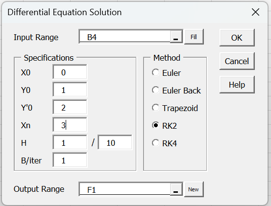
Figure 3 – Dialog box for 2nd order differential equation
After clicking on the OK button, the output in Figure 4 appears.
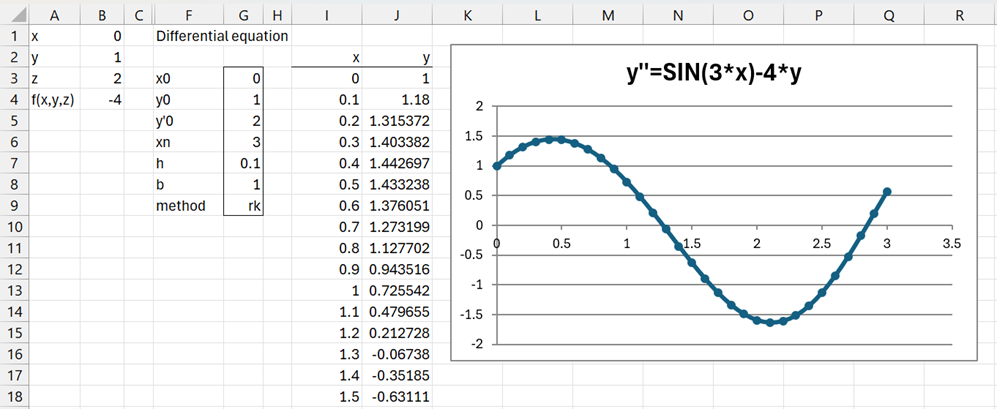
Figure 4 – Differential equation solution
Note that since you are solving a second-order differential equation, you need to specify a numeric value for Y′0 in the dialog box. You can change this value to a different number in the output (cell E5 of Figure 4), and all values will be adjusted automatically. If you change the value to a blank, this will be treated as a zero.
Worksheet Function
The Chart Title (in Figures 2 and 4) describes the differential equation using the following worksheet function provided in the Real Statistics Resource Pack.
EvalSymbolic(R1, ttype, Rx, Ry, Rz): returns the expression in R1 substituting the letters x, y, z for the cell addresses in R1.
R1 contains an expression that represents a function in 1, 2, or 3 values. R1, Rx, Ry, and Rz are as described for DiffEq2 in Second Order Differential Equations.
ttype takes the values -2, -1, 0, 1, or 2. If ttype = 0, a string of the form f(…) = … is returned. If ttype = 2 then a string of form y′′ = … is returned (any z on the right-hand side is replaced by y′), while if ttype = 1 then a string of form y′ = … is returned. When ttype = -2 0r -1 then the same text is returned as for –ttype without the y′′ or y′ part on the left side of the output.
Figure 5 shows various examples of the use of this function to help explain things more clearly.
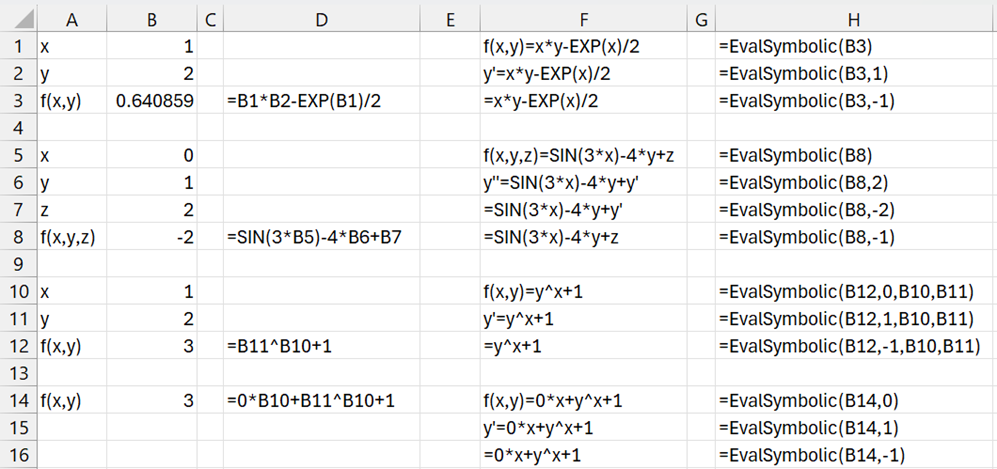
Figure 5 – EvalSymbolic examples
Examples Workbook
Click here to download the Excel workbook with the examples described on this webpage.
Links
↑ Numerical differential equations
References
Strang, G., Herman, E., Seeburger, P. (2025) Introduction to differential equations
https://math.libretexts.org/Courses/Monroe_Community_College/MTH_211_Calculus_II/Chapter_8%3A_Introduction_to_Differential_Equations/8.1%3A_Basics_of_Differential_Equations
Atkinson, K., Han, W., Stewart, D. (2009) Numerical solutions to ordinary differential equations. Wiley-Interscience
https://homepage.math.uiowa.edu/~atkinson/papers/NAODE_Book.pdf
Hossain, J., Alam, S., Hossain, B. (2017) A study on numerical solutions of second order initial value problems (IVP) for ordinary differential equations with fourth order and Butcher’s fifth order Runge-Kutta methods
http://article.sapub.org/10.5923.j.ajcam.20170705.02.html
Wikipedia (2025) Numerical methods for ordinary differential equations
https://en.wikipedia.org/wiki/Numerical_methods_for_ordinary_differential_equations