On this webpage, we extend the results about local maxima and minima from Maxima/Minima of a Function about a continuous function f(x) in one variable to continuous functions f(x, y) and f(x, y, z) in two or three variables.
Basic Concepts for Two-variable Functions
To determine the local maxima or minima of a continuous function f(x,y) with two variables, we first need to calculate the two partial derivatives of the function, one with respect to x and the other with respect to y. The 2 × 1 vector of such values is called the gradient. Values of x and y where these partial derivatives are both zero are called critical values or critical points. These are our candidates for local maxima and minima. In fact, to determine whether a critical value is a local maximum or a local minimum, we must look at the 2 × 2 matrix of second-order partial derivatives, called the Hessian matrix.
For those of you who are familiar with calculus, the gradient and Hessian are defined as
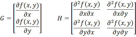
Since the two off-diagonal elements of the Hessian matrix H = [hij] are equal, this is a symmetric matrix. Also, note that the determinant D of H is
![]()
Critical Points
It turns out that a critical point can be characterized as follows:
- If D > 0 and h11 > 0, then x,y is a local minimum
- If D > 0 and h11 < 0, then x,y is a local maximum
- When D < 0 then x,y is a saddle point (two-dimensional version of an inflection point)
- When D = 0 then x,y is indefinite (i.e. you can’t tell which type of critical value it is from using H)
For those of you who are familiar with linear algebra, if H is positive-definite then we have a local maximum and if H is negative-definite then we have a local minimum. This turns out to be equivalent to the test that if H’s eigenvalues are positive then we have a local maximum, if they are negative then we have a local minimum, while if the signs are different, then we have a saddle point. These criteria also hold for higher dimensional Hessian matrices.
Basic Concepts for Three-variable Functions
The situation is similar for continuous function f(x,y,z) in three variables. A critical point occurs when the three partial derivatives are zero. Once again, a critical point can be a local maximum, a local minimum, or a saddle point. We use the 3 × 3 Hessian matrix of second-order partial derivatives to determine which type of critical value we have. If D is the determinant of the Hessian matrix and E is the determinant of the upper 2 × 2 portion of the Hessian matrix, then the rules are:
- When E > 0 and D > 0 & h11 > 0, then x,y,z is a local minimum
- When E > 0 and D < 0 & h11 < 0, then x,y,z is a local maximum
- If D = 0 then x,y,z is indefinite
- Otherwise, x,y,z is a saddle point
Worksheet Functions
The following worksheet functions take lambda function parameters. These are described in Real Statistics Lambda Capabilities and Lambda Functions using Cell Formulas.
Real Statistics Functions: The Real Statistics Resource Pack provides the following worksheet functions that identify a local minimum and maximum of a function in two variables x and y.
MNEWTON2(R1, guessx, guessy, iter, prec, incr, Rx, Ry): returns a 2 × 4 array containing the values x, y that identify a possible local maxima or minima of f(x, y), based on Newton’s method using the initial guesses guessx for x and guessy for y.
R1 is a cell that contains a formula that represents the function f(x, y) and the addresses of cell Rx and Ry reference the variables x and y in R1. If Rx and Ry are omitted, they default to the first and second cells referenced in R1. See Lambda Functions using Cell Formulas for more details and other options for R1, R2, and Rx.
iter (default 100) = the maximum number of iterations. The algorithm will terminate prior to iter iterations if the error is less than some value based on prec (default .0000001).
Since this approach uses the Real Statistics function DERIV to estimate the partial derivatives of the function f(x, y), the incr parameter used by DERIV needs to be specified (default .000001); See Numerical Differentiation.
The first column of the output contains the values x and y of a critical point. The second column contains the values of the partial derivatives of f(x,y) at these values (which should be close to zero if there is convergence). Next, the third column contains the value f(x,y) and the type of critical value (local maximum, local minimum, saddle point, or indeterminate). The rest of the output contains the 2 × 2 Hessian matrix.
Three variable case
The following worksheet function performs a similar role for three variable functions.
MNEWTON3(R1, guessx, guessy, guessz, iter, prec, incr, Rx, Ry, Rz): returns a 3 × 5 row array containing the values x, y, z that identify a local maxima or minima of f(x,y,z) based on Newton’s method using the initial guesses guessx for x and guessy for y and guessz for z. The output is similar to that from MNEWTON2.
Examples for f(x,y)
Example 1 (min/max)
Find local maxima and minima for the function f(x,y) = x2 + y2 – xy for the initial guess shown in Figure 1.
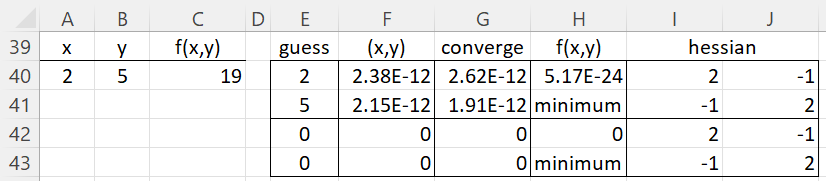
Figure 1 – Local minimum for f(x,y)
The function under consideration is shown in cell C40 which contains the formula =A40^2+B40^2-A40*B40. We first consider the initial guesses x = 2 (cell E40) and y = 5 (cell E41). Using the array formula =MNEWTON2(C40,E40,E41) in range F40:J41, we obtain the critical point of (2.38E-12, 2.15E-12) as shown in cells F40 and F41. Given the roundoff error, this is likely to be the point (0,0), which is confirmed by the second guess in range E42:E43.
Since the values in cells G40 and G41 are close to zero, we see that the algorithm converges to a solution. Since the determinant of the Hessian shown in range I40:J41 is 2⋅2 – (-1)(-1) = 3, which is negative, the critical value is either a local minimum or a local maximum. Finally, since the first element in the Hessian is 2, which is positive, the critical point is a local minimum, as shown in cell H41.
Example 2 (saddle point)
Find local minima and maxima for the function f(x,y) = xex – y3 + ln y for various initial guesses, as shown in Figure 2.
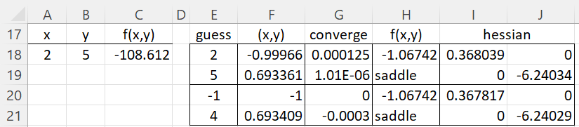
Figure 2 – Critical points for f(x,y)
The function under consideration is shown in cell C18 which contains the formula =A18*EXP(A18)-B18^3+LN(B18). We first consider the initial guesses x = 2 (cell E18) and y = 5 (cell E19). Using the array formula =MNEWTON2(C18,E18,E19) in range F18:J19, we obtain a critical point of (-.99966, .693361) as shown in cells F18 and F19. Given the roundoff error, this is likely to be the point (-1, .6934).
Since the values in cells G18 and G19 are close to zero, we see that the algorithm converges to a solution. Since the determinant of the Hessian shown in range I18:J19 is negative, the critical value is a saddle point.
Note too that the second guess of (-1, 4) yields a similar result.
Example 3 (indefinite)
Determine whether the function f(x,y) = x2 + y4 has a critical value at the origin, and if so which type of critical value it is.
From Figure 3, we see that (0,0) has a critical value (since column G contains two zeros). Furthermore, we see that the determinant of the Hessian is zero and so the type of critical value can’t be determined by using the Hessian.
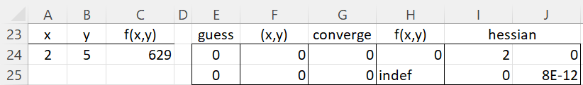
Figure 3 – Indeterminate critical value for f(x,y)
But since we know that f(x,y) = x2 + y4 is always positive except at the original where it is zero, we conclude that a local minimum occurs at (0, 0).
In general, we can determine the type of critical at (x,y), by looking at the function values for points close to (x,y). E.g. for some small positive value h, if f(x+h,y) > f(x,y) and f(x,y+h) > f(x,y) and f(x+h,y+h) > f(x,y), then a critical value at (x,y) is likely to be a local minimum. If the three inequalities are all < instead of > then the critical value is likely to be a local maximum. If there is a mix of > and < then we likely have a critical value.
Example for f(x,y,z)
Example 4: Find local minima and maxima for the function f(x,y,z) = x3 + y2 + 2z2 + xz2 – 3x2 for the initial guesses shown in Figure 4.
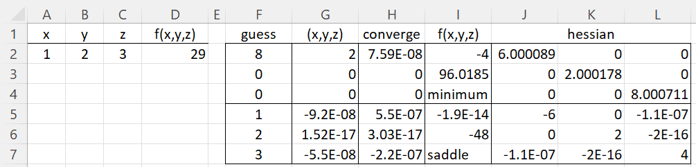
Figure 4 – Critical values for f(x,y,z)
The function under consideration is shown in cell D2 which contains the formula A2^3+B2^2+2*C2^2+A2*C2^2-3*A2^2. We first consider the initial guesses (8, 0, 0). Using the array formula =MNEWTON3(D2,F2,F3,F4) in range G2:L4, we obtain a critical point of (2, 0, 0) as shown in cells F18 and F19.
Since the values in cells H2, H3, and H4 are close to zero, we see that the algorithm converges to a solution. We see that the determinant of the Hessian is 96 (cell I3), the determinant of the upper 2 × 2 portion of the Hessian is 6⋅2-0⋅0 = 6 and the first entry in the Hessian is 6 (cell J6). Since all three of these values are positive, we conclude that the critical value is a local minimum, as confirmed by the entry in cell I4.
For the second guess of (1, 2, 3), we obtain a critical value of (0, 0, 0). Since the determinant of the Hessian is -48, which is not zero, and the determinant of the upper 2 × 2 portion of the Hessian is (-6)⋅2-0⋅0 = -6, which is negative, we conclude that (0, 0, 0) is a saddle point, as confirmed in cell I7.
Examples Workbook
Click here to download the Excel workbook with the examples described on this webpage.
Links
↑ Min/max of a continuous function
References
Fabretti, A. (2015) Function of several variables, quadratic forms and optimization
https://economia.uniroma2.it/ba/business-administration-economics/corso/asset/YTo0OntzOjI6ImlkIjtzOjM6IjgyMCI7czozOiJpZGEiO3M6NToiMTkyNzIiO3M6MjoiZW0iO047czoxOiJjIjtzOjU6ImNmY2QyIjt9
Math Help Boards (2012) Extrema points, a function of three variables
The link is no longer active
Schlicker, S. (2021) Optimization. Active Calculus.
https://activecalculus.org/multi/S-10-7-Optimization.html
Lebl, J. (2017) The Hessian and optimization
https://math.okstate.edu/people/lebl/osu4013-s17/hessian.pdf