Proportional Odds Model Proofs

Property 1: The maximum value of the log-likelihood function LL occurs when the following r+k-1 equations hold for h = 1 to r-1.

or alternatively

and for j = 1 to k

where

Proof

The likelihood function is maximized when the first partial derivatives of LL with respect to the a_h are zero for h = 1 to r-1 and the first partial derivatives of LL with respect to the b_j are also zero for j = 1 to k. We define the following:

Thus

We also note that for 1 < h < r

from which it follows that

For h = 1 and h = r, we have

We next calculate various partial derivatives

For 1 < h < r, we have

For h = 1 and h = r, we get

Since p_i0 = 0 and p_ir = 1, even when h = 1 or h = r

And so this result holds for 1 ≤ h ≤ r.

For 1 < h < r, we have

For h = 1, we have

and so for 1 ≤ h ≤ r-1

We next consider

which is valid for 0 < h < r-1. It is also valid for h = r-1 as can be seen from

We also note that

Finally, we now calculate the partial derivatives of LL using the results described above.

Since

it follows that for 0 < h < r

which completes the proof.

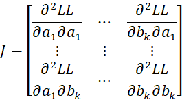
Property A: The Jacobian matrix of the second partial derivatives of LL is an k+r-1 × k+r-1 symmetric matrix of form

where C = [c_hl] is an r-1 x r-1 matrix, D = [d_jg] is a k × k matrix and U = [u_jh] is an k × r-1 matrix consisting of the following elements:

where

Proof

We calculate the various second partial derivatives of LL using the properties described in the proof of Property 1. We start with the 

terms.

Next, we calculate the

terms.

Finally, we have the case. First, we note that

which is also true in the following two cases:

We now start with the case where l = h.

If l = h + t where t ≥ 2, then

and so

Finally, we consider the case where  and 0 < h < r-1, but first we note that

It now follows that

This completes the proof.

Property 2 (Newton’s method)

Proof: Let

Using Newton’s method, we conclude that B* is a better estimate of the regression coefficients than B (i.e. it produces a larger value for LL), and so the sequence B, B*, B**, B***, etc. converges to the coefficient vector that maximizes LL and the corresponding Hessian matrix J^-1 is a good estimate of the covariance matrix for the regression coefficients.

From Property 1, we see that the F vector can be expressed as

where

and by Property A, we see that the Jacobian matrix can be expressed as 

where C = [c_hl], D = [d_jg] and U = [u_jh] are as described in Property A. This completes the proof.

References

Hyun Sun Kim (2004) Topics in ordinal logistic regression and its applications. Dissertation Texas A & M
No longer accessible online
Agresti, A. (2013) Modeling Ordinal Categorical Data tutorial
http://statmath.wu.ac.at/research/talks/resources/slidesagresti_ordinal.pdf
McCullagh, P. (1980) The proportional odds model
https://www.stat.uchicago.edu/~pmcc/reports/prop_odds.pdf