We now use the NIPALS algorithm to find the PLS regression coefficients for the simple example taken from the Abdi (2003) reference.
Example
Example 1: Create a PLS regression model for the data in Figure 1. Here Hedonic measures the taste, Meat measures how well the wine goes with meat, and Dessert measures how well the wine goes with dessert.
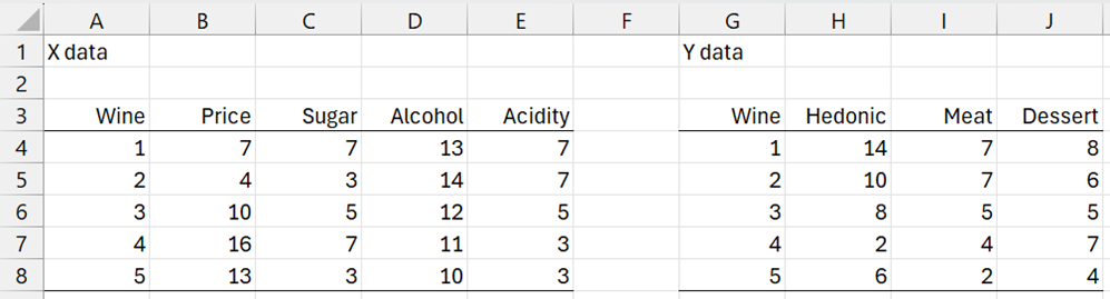
Figure 1 – Wine data
First, we note that there are two problems when trying to perform linear regression using the X data in range B4:E8 and the Y data in any other columns in G4:H8. First of all, there is the likelihood of multicollinearity since the correlation between Acidity and Alcohol is about 95% and between Price and Acidity about -95%, and between Price and Alcohol about -90%.
Secondly, there are 4 independent variables and only 5 data vectors, which means that you need at least one more row of data if your regression model contains an intercept.
Initialization
Standardizing the columns and initializing u with the values in range H13:H17, we obtain the results in Figure 2. E.g. we obtain the values in column B13:B17 by inserting the Real Statistics formula =XSTANDARDIZE(B4:B8) in range B13:B17.
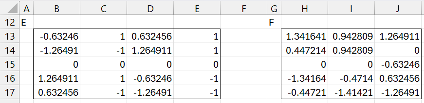
Figure 2 – Initialization
Iteration 1
We now calculate the vectors w, t, c, u, as described in PLS Regression Basic Concepts. Convergence occurs after 8 iterations, as shown in Figure 3.
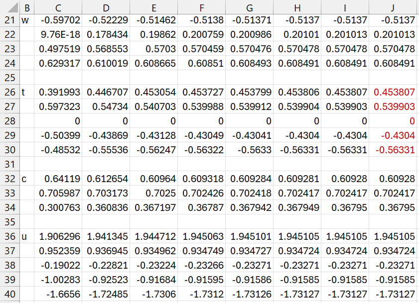
Figure 3 – First inner loop
We insert the following array formula in range C21:C24
=NORM(MMULT(TRANSPOSE($B13:$E17),H13:H17))
The subsequent w vector values are computed by inserting the formula
=NORM(MMULT(TRANSPOSE($B13:$E17, B36:B40)
in range D21:D24, highlighting range D21:J24, and pressing Ctrl-R.
The t, c, and u vectors are computed by inserting the formulas
=MMULT($B13:$E17,C21:C24) in range C26:C30
=NORM(MMULT(TRANSPOSE($H13:$J17),C26:C30)) in range C32:C34
=MMULT($H13:$J17,C32:C34) in range C36:C40
and then highlighting range C26:J40 and pressing Ctrl-R.
The converged values for w, t, c, and u are shown in range J21:J40.
We now calculate d and p, as shown in Figure 4.
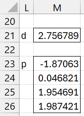
Figure 4 – d and p
Cell M21 contains the array formula =MMULT(TRANSPOSE(J26:J30),J36:J40) and range M23:M26 contains the array formula =MMULT(TRANSPOSE(B13:E17),J26:J30).
Next, we deflate E and F, as shown in Figure 5.
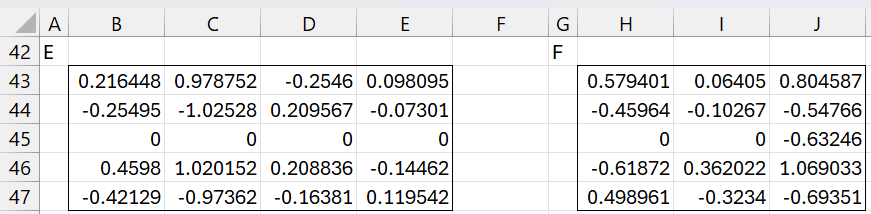
Figure 5 – Deflated E and F matrices
Here, range B43:E47 contains the formula
=B13:E17-MMULT(J26:J30,TRANSPOSE(M23:M26))
and H43:J47 contains the formula
=H13:J17-M21*MMULT(J26:J30,TRANSPOSE(J32:J34)
Iteration 2
We now repeat the calculations shown in Figures 3 and 4, starting with the E and F matrices displayed in Figure 5 instead of those shown in Figure 2. The results are shown in Figures 6 and 7. This time convergence occurs after 6 steps.
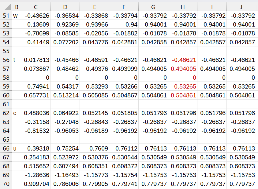
Figure 6 – w, t, c, u for iteration 2
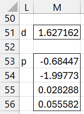
Figure 7 – d and p for iteration 2
Iteration 3
We now deflate the E and F matrices once again and calculate w, t, c, u, d, p as before. If we deflate E another time we will obtain the null matrix. Deflating F another time results in a matrix the first two columns of which are null.
Termination
We now define the W, T, C, U, and P matrices by concatenating the corresponding w, t, c, u, and p vectors for each of the three iterations. In addition, we create a diagonal matrix D whose main diagonal consists of the three d values. The result is shown in Figure 8.
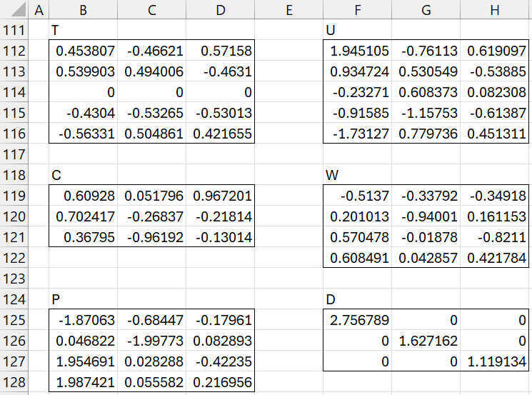
Figure 8 – W, T, C, U, P, D matrices
Note that the values in the first column of T (range B112:B116) are the same as those in range J26:J30. Similarly, the values in the second column (range C112:C116) are the same as those in range J56:J60. The values in the third column are derived from the t vector in the third iteration. The same is true for the other matrices in Figure 8.
Note that the columns in the T and U matrices are mean centered (i.e. mean = zero). Also, the columns in T, W, and C have unit length.
Decomposition
We now calculate the matrices TP′ and TDC′, as shown in the upper part of Figure 9.
The values in range B133:E137 are calculated by the formula
=MMULT(B112:D116,TRANSPOSE(B125:D128))
The values in range G133:I137 are calculated by the formula
=MMULT(B112:D116,MMULT(F125:F127,TRANSPOSE(B119:D121)))
Note that X = TP′ and the first two columns of Y are the same as those of TDC′.
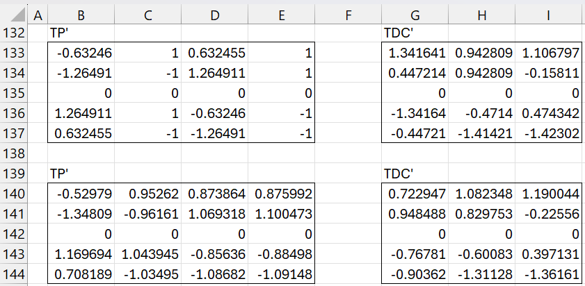
Figure 9 – Estimates for X and Y
The lower part of Figure 9 is based on the 2 latent vector model instead of the 3 latent vector model. Thus, range B140:E144 contains the formula
=MMULT(B112:C116,TRANSPOSE(B125:C128))
and range H140:J144 contains the formula
=MMULT(B112:C116,MMULT(F125:G126,TRANSPOSE(B119:C121)))
Regression Coefficients
The standardized regression coefficient matrix
B = (P′)+DC′
is calculated as shown in Figure 10.
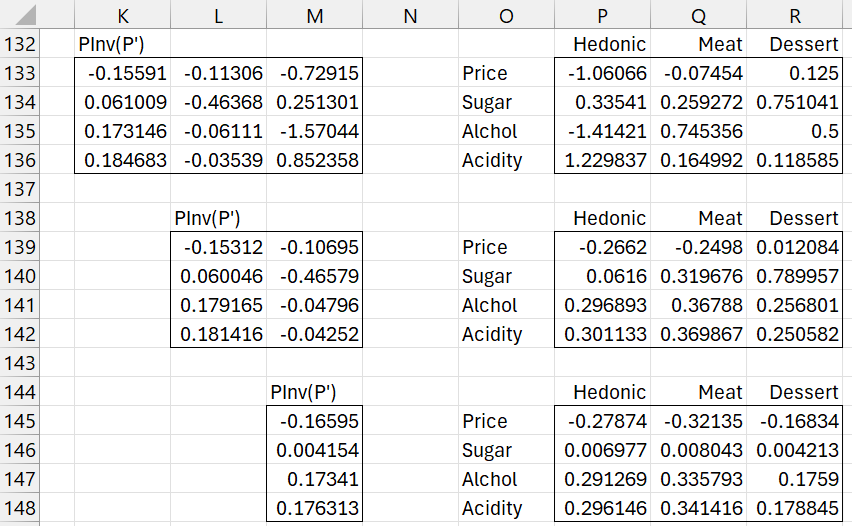
Figure 10 – Standardized PLS regression coefficients
For the 3 latent vector model, the regression coefficient matrix, shown in range P133:R136, is calculated by
=MMULT(K133:M136,MMULT(F125:F127,TRANSPOSE(B119:D121)))
where the pseudo-inverse (P’)+ in K133:M136 is calculated by
=PseudoInv(TRANSPOSE(B125:D128))
The regression coefficient based on the 2 latent vector model is shown in range P139:R142 and the result with 1 latent vector is shown in range P145:R148.
We now need to find the equivalent unstandardized coefficients. First we calculate the mean and standard deviations for all the columns in X and Y. This is shown in Figure 11.
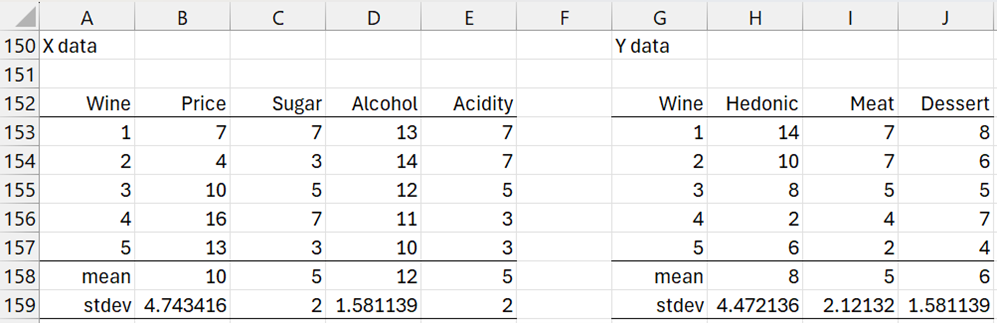
Figure 11 – Means and standard deviations
The (unstandardized) PLS regression coefficients for 3, 2, and 1 latent vectors are shown in Figure 12.
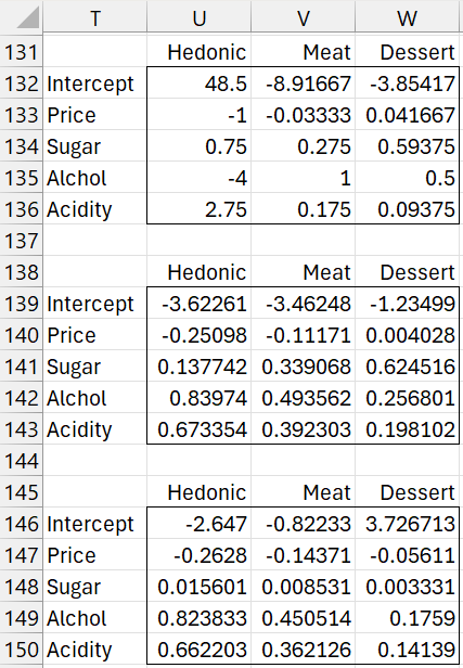
Figure 12 – Unstandardized PLS regression coefficients
For the 3 latent vector model shown in range T131:W143, we inserted the array formula
=H159:J159*P133:R136/TRANSPOSE(B159:E159)
in range U133:W143 and
=H158:J158-MMULT(B158:E158,U133:W136)
in range U132:W132.
Examples Workbook
Click here to download the Excel workbook with the examples described on this webpage.
References
Hervé Abdi (2003) Partial least squares (PLS) regression
https://www.utdallas.edu/~herve/Abdi-PLS-pretty.pdf