Basic Concepts
While Ridge regression addresses multicollinearity issues, it is not so easy to determine which variables should be retained in the model. These variables will converge to zero more slowly as lambda is increased, but they never get to zero.
LASSO, which stands for least absolute selection and shrinkage operator, addresses this issue since with this type of regression, some of the regression coefficients will be zero, indicating that the corresponding variables are not contributing to the model. This is the selection aspect of LASSO. Thus, LASSO performs both shrinkage (as for Ridge regression) but also variable selection. In fact, the larger the value of lambda, the more coefficients will be set to zero.
For LASSO regression, we add a different factor to the ordinary least squares (OLS) SSE value as follows:
Properties
There is no simple formula for the regression coefficients, similar to Property 1 of Ridge Regression Basic Concepts, for LASSO. Instead, we use the following iterative approach, known as cyclical coordinate descent.
First, we note that this iterative approach can be used for OLS regression. This is based on the following property.
Observation: In the cyclical coordinate descent algorithm, initially set all the bj to some guess (e.g. zero) and then calculate b0, b1, …, bk as described in Property 1. Continue to do this until convergence (i.e. the values don’t change more than a predefined amount).
We use the same approach for LASSO, except that this time we use the following property.
Property 2:
where cj and zj are defined as in Property 1.
Observation: Initially set all the bj = 0 and then calculate c0, b0, c1, b1, …, ck, bk as described in Property 2. Continue to do this until convergence (i.e. the values don’t change more than a predefined amount).
Worksheet Function
Real Statistics Function: The Real Statistics Resource Pack provides the following functions that implement this algorithm.
LASSOCoeff(Rx, Ry, lambda, iter, guess) – returns a column array with standardized LASSO regression coefficients based on the x values in Rx, y values in Ry, and designated lambda value using the cyclical coordinate descent algorithm with iter iterations (default 10000) and with the initial guesses for each coefficient as specified in the column array guess; alternatively guess can specify a single initial value for all the coefficients (default .2)
Note that Rx and Ry are the raw data values and have not yet been standardized.
Example
Example 1: Find the LASSO standardized regression coefficients for various values of lambda. Use these to create a LASSO trace and determine the order in which the coefficients go to zero.
The results are shown in Figure 1.
Figure 1 – LASSO Trace
For example, the array worksheet formula in range I4:I7 is =LASSOCoeff($A$2:$D$19,$E$2:$E$19,I3). We see that X2 is the first variable to go to 0, followed by X4, X3, and X1. It is not hard to see that these happen at about lambda = .14, 1.05, 12.6, and 32.7.
The LASSO Trace is then constructed using Excel’s line charting capability based on the data in range G3:N7.
Data Analysis Tool
The Real Statistics Resource provides the LASSO Regression data analysis tool.
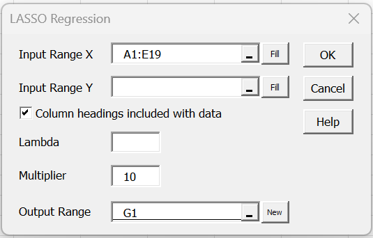
To use this tool for Example 1, press Ctrl-m, and select the LASSO Regression option from the Reg tab. Fill in the dialog box that appears as shown in Figure 2. Here, we elected to leave the Lambda field blank to accept the default.
Figure 2 – LASSO Regression dialog box
After pressing the OK button, output similar to that shown in Figure 1 will be displayed.
Examples Workbook
Click here to download the Excel workbook with the examples described on this webpage.
Reference
Penn State (2018) The Lasso. Applied Data Mining and Statistical Learning
https://online.stat.psu.edu/stat857/node/158/


Hello sir,
Ridge regression is provided via GUI, but LASSO is not. Is there going to be a GUI version of LASSO regresion in the future? Or any plans to extend current Ridge regerssion GUI to be able to use both Ridge and LASSO terms (L1 and L2 regularization)?
Hi Brian,
Thanks for your comment.
I plan to add LASSO support to the GUI interface shortly, probably the next full release.
As far as the rest, I need to look into this. Do you have a good reference that I can use?
Charles