Introduction
We now review the support that Real Statistics provides for carrying out coarsened exact matching (CEM). This support is provided via the Coarsened Exact Matching data analysis tool.
Reference will be made to various worksheet functions.
Coarsening the Data
The Coarsened Exact Matching data analysis tool works by first creating bins (as for a histogram) for each of the confounding variables. This is done by using the following new worksheet function:
CEM_Coding(R1, R2)
R1 is an array with column headings in the first row whose first column contains zeros and ones where 1 corresponds to the treatment group and 0 corresponds to the control group. The other columns contain sample data for one confounding variable. The data has been sorted so that the rows corresponding to the control group occur before the rows containing data from the treatment group. R2 is an array that contains codes that fix the bins.
Coding Example
For example, suppose that R1 contains data for three confounding variables: Age, Gender, and Test score. Also suppose that Age is binned as 1 = 0-20, 2 = 21-40, 3 = 41-60, 4 = 60+; Gender is binned as 0 = female and 1 = male; and Score is binned as 1 = 0-19, 2 = 20, 3 = 21+. In this case, R2 could contain the data in range A1:B4 of Figure 1.
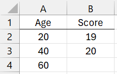
Figure 1 – Coding Example
The column headings are needed to match with the column headings in the data in R1. Here the first entry for Age is 20, which means that code 1 (all such codes begin with 1) and signifies age ≤ 20. The next entry takes code 2 and signifies 20 < age ≤ 40. The last entry takes code 3 and signifies 40 < age ≤ 60. Any age > 60 is coded as 4.
Similarly, a score ≤ 19 takes code 1, a score = 20 takes code 2, and any score > 20 takes code 3. Finally, any variable not in R2 takes a code equal to its value. For this example, gender = 0 takes code 0 and gender = 1 takes code 1.
Creating Bin Signatures
The output from CEM_Coding(R1, R2) contains the coding for all the values in R1, excluding the first column, based on the coding in R2. A copy of this output is then sorted eliminating duplicates, using the existing array function SortsRowsUnique, to obtain a set of patterns (rows in the output) called bin signatures.
Next, each each row in the output from CEM_Coding(R1, R2) is assigned a bin signature index. This is done via the worksheet function:
RowMatch(R1, R2)
R1 is an array each of whose rows consists of the bin signatures. R2 is a row from the output from the coarsening process. The output from this function consists of the matching bin signature index; i.e. the row number of the bin signature that matches the bin signature in R1. If no such match is obtained then the output is zero.
Using this function for each row R2 from the output from the coarsening process, the data analysis tool obtains a column of bin signature indices for each coarsened row from the original data array. Let’s refer to this column array as R0.
Weights
Next, each row in the bin signature array is assigned a weight, as described in Coarsening Exact Matching. Let’s call the column array consisting of all such weights Rw.
These weights are now transferred to a new column array, which we will call R2, next to the column array referred to as R0 above by using the formula =IF(C0=0,0,INDEX(C0, Rw)) for each cell C0 in column array R0.
Once we have assigned the weights, the array of coarsened data has served its purpose and we go back to looking at the original, uncoarsened data and the corresponding weights in R2.
Pruning
Just as we did for Propensity Score Matching, we now prune any unmatched data rows (corresponding to a zero in the bin or weight column array) using the worksheet function
Pruning(R1, R2, b)
R1 is an array containing the original data (for confounding variables as well as the outcome variable) and R2 is the column array consisting of weights for the data in R1. This time we set b = TRUE (default), which means the output consists of all matched rows from R1 (eliminating any unmatched row, i.e. where the weight = 0), augmented with the row of weights as its last column.
Match Quality
Finally, we can elect to look at the quality of matching via the function:
MatchQuality(R1, b)
R1 is an array containing data for the treatment variable (with values 0 or 1), any confounding variables and the outcome variable, and the weights. The first column of R1 contains the data for the treatment variable and the last column contains the weights.
This function is defined more completely in Propensity Score Matching. For Coarsened Exact Matching, however, the second argument b is set to FALSE, which means that the last two rows of the output are not included, and the entries in the output are calculated using the weights.
Note that inspecting the matching quality is less important for CEM compared to PSM, since we expect better matching from CEM.
Example
Click here for an example that shows how all the steps fit together.
1-to-1 Matching
Weights are important to the approach described on this webpage. Click here for a description of a version of CEM that doesn’t rely on weights.
This approach uses the following additional worksheet function:
CEM_Pairing(R1, R2)
R1 is a column array containing bin signature indices and R2 is a two-column array with one row for each bin signature. Each row of R2 contains the count of treatment subjects that match the bin signature corresponding to that row and the count of control subjects that match the bin signature for that row.
The output from this function is a column array with the same number of rows as R1 that contains zeros and ones. One indicates that the corresponding subject is retained, while a zero indicates that the corresponding subject is pruned.
Links
References
King, G. (2015) Why propensity scores should not be used for matching
https://www.youtube.com/watch?v=rBv39pK1iEs
Huntington-Klein, N. (2012) Coarsened exact matching and entropy balancing
https://www.youtube.com/watch?v=M6AsS4zaWQk
Blackwell, M., Iacus, S., King, G., Porro, G. (2011) CEM for SPSS
https://projects.iq.harvard.edu/cem-spss/pages/how-use-cem-spss
Huffman, A. (2017) CEM: Coarsened exact matching explained
https://medium.com/@devmotivation/cem-coarsened-exact-matching-explained-7f4d64acc5ef
Wu, W. (2023) Coarsened exact matching
https://cem-linearinf.readthedocs.io/en/latest/tuto_cem.html
Wu, W. (2023) Balance checking
https://cem-linearinf.readthedocs.io/en/latest/tuto_balance.html
Wu, W. (2023) Inference
https://cem-linearinf.readthedocs.io/en/latest/tuto_inf.html
Wu, W. (2023) Sensitivity analysis
https://cem-linearinf.readthedocs.io/en/latest/tuto_sen.html