Example
Example 1: Find the eigenvalues and eigenvectors for the symmetric matrix in range A3:D6 of Figure 1, where cells D3 and A6 contain the formula =SQRT(2).
Figure 1 – Eigenvalues with multiplicity > 1
In this example, we see that the eigenvalue 2 is repeated twice. Also, the corresponding eigenvectors corresponding to 2 are the same and so this time the eigenvectors are not orthogonal. This can be repaired by solving the homogeneous linear equation (A–λI)X = 0 where A is the matrix in range A3:D6 and λ = 2, as shown in Figure 2.
Figure 2 – Finding orthogonal eigenvectors
The homogeneous linear equation is shown in range F12:J15 where the values in range F12:I15 are calculated via the array formula =A3:D6-G3*Identity(4). As explained in Multiple Solutions to Linear Equations, all solutions X to this set of linear equations can be expressed as a linear combination of the vectors in L12:L15 and M12:M15. The first of these vectors is already one of the eigenvectors associated with λ = 2, while the second vector is a distinct eigenvector for λ = 2. The equivalent vector with length 1 is shown in range P12:P15.
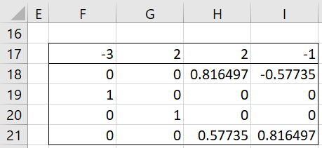
If we substitute this vector for the eigenvector in range H4:H7 of Figure 1, then we get the eigenvectors shown in Figure 3.
Figure 3 – Orthogonal eigenvectors
It turns out that these eigenvectors are orthogonal since the worksheet array formula =MMULT(MINVERSE(F18:I21),F18:I21) outputs the identity matrix. Thus, the matrix in range F18:J21 is orthonormal (as described in Orthogonal Vectors and Matrices).
Note that when the resulting vectors are not orthogonal, we can use the QRFactorQ function described in QR Factorization to obtain equivalent eigenvectors that are orthogonal. For Example 1, this would be produced via the formula =QRFactorQ(L12:M15).
Perturbance approach
Another approach to finding orthogonal eigenvectors is to perturb one or more elements in the original matrix so that the repeated eigenvalues separate just a little. In this way, the corresponding eigenvectors will become distinct. This approach is illustrated in Figure 4.
Figure 4 – Perturbing the original matrix
When the value in cell C14 is changed from 2 to 2.00001, we obtain the same eigenvectors that we obtained in Figure 6. We would obtain similar results if we perturbed the value in cells A12, D15, D12 or A15. We don’t get the desired result if we perturb the value in cell B13 since this results in a change to the -3 eigenvalue and not the 2 eigenvalue. Perturbing any of the other cells also doesn’t get us the desired result. If, however, we perturb both the B12 and A13 cells by the same amount, we once again obtain the eigenvectors shown in Figure 3.
Defective eigenvalues
Not all repeated eigenvalues will have m independent eigenvectors where m is the multiplicity of the eigenvalue. Such eigenvalues are called defective.
Example 2: Find the eigenvalues and eigenvectors for the matrix in range A2:B3 of Figure 5.
Figure 5 – Defective eigenvalue
We see from D2:E3 that this matrix has one repeated eigenvalue, namely -1 with multiplicity 2. We set up the homogenous linear equation in range G2:I3 and find in range K2:K3 that there is only one independent unit eigenvector, namely that shown in D3:D4 (or E3:E4 or N2:N3), all others eigenvectors are scalar multiples of this one.
Symmetric matrix
A symmetric matrix cannot have a defective eigenvalue (see Property 2 of Spectral Decomposition). Thus, even if there is a repeated eigenvalue, say of multiplicity m, you can still find m orthogonal unit eigenvectors corresponding to this eigenvalue.
Also, note that eigenvectors corresponding to distinct eigenvalues of a symmetric matrix are orthogonal (see Property 2 of Symmetric Matrices). Thus, for any n × n real symmetric matrix, there are n orthogonal real eigenvectors corresponding to the n real eigenvalues.
Worksheet Function
Real Statistics Function: The Real Statistics Resource Pack provides the following function to find orthogonal eigenvectors corresponding to a non-defective eigenvalue.
eigMultVECT(R1, lambda, prec): outputs an array whose columns are mutually orthogonal eigenvectors corresponding to the eigenvalue lambda for the square matrix R1; prec is a small positive number (default .0001) where values ≤ prec are treated as if they were zero.
Examples Workbook
Click here to download the Excel workbook with the examples described on this webpage.
References
Golub, G. H., Van Loan, C. F. (1996) Matrix computations. 3rd ed. Johns Hopkins University Press
Searle, S. R. (1982) Matrix algebra useful for statistics. Wiley
Perry, W. L. (1988) Elementary linear algebra. McGraw-Hill
Fasshauer, G. (2015) Linear algebra.
https://math.iit.edu/~fass/532_handouts.html
Lambers, J. (2010) Numerical linear algebra
https://www.yumpu.com/en/document/view/41276350


