Using Iterative Search
We can estimate the parameter values of a PERT distribution that fits the data in a data set by iterative search in the same manner as we did for the triangular distribution. We won’t go into all the details of how to do this, but instead, explain the PERT_FITM that implements this approach.
Worksheet Function
Real Statistics Function: The Real Statistics Resource Pack provides the following worksheet function that estimates the parameters of a PERT distribution that fits the data in R1 based on the method of moments.
PERT_FITM(R1, lab, lo, hi, iter, exta, extb, iterb, iterc): returns a column array with the estimated values of the parameters a, b, c; along with the mean, variance, and skewness based on the data in R1 and the distribution parameters; and finally the MLE and the sum of squares.
The arguments are exactly as for TRIANG_FITM (see Method of Moments: Triangular Distribution).
Example (Iterative Search)
Example 1: Repeat Example 1 of Method of Moments: PERT Distribution using the PERT_FITM function.
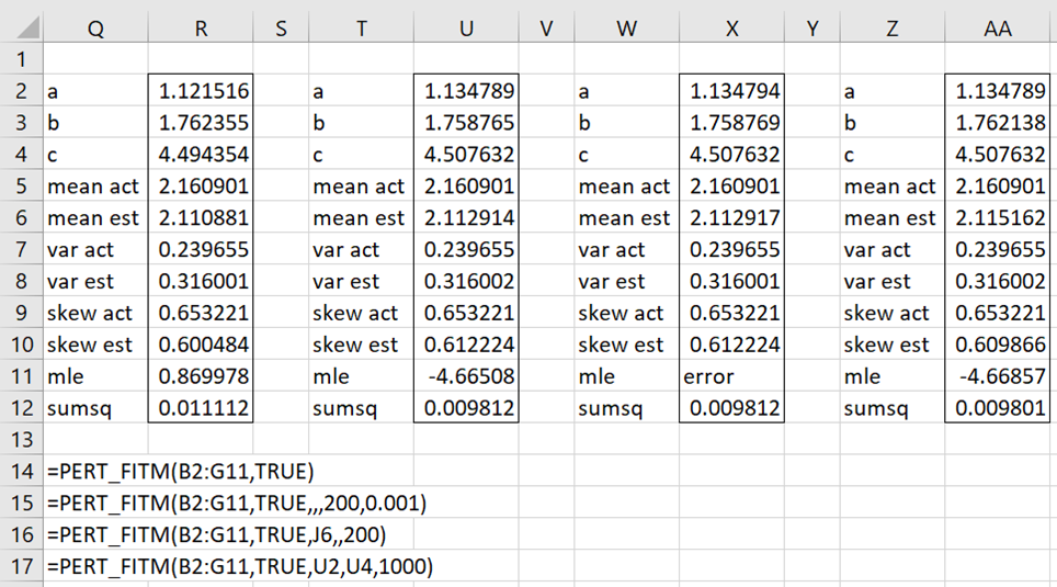
We use the formula =PERT_FITM(B2:G11,TRUE) to obtain the results shown in range Q2:R12 of Figure 1. These values are similar to, but not exactly the same as, the values in Figure 4 of Method of Moments: PERT Distribution. Note that the sum of squares (cell D14 in Figure 4 of that webpage) is not quite as good as the equivalent value in Figure 1 below, but the MLE (cell R11) exists since the PERT_FITM formula guarantees that the boundary conditions (a < min, max < c, a < b < c) are met.
Figure 1 – Using PERT_FITM
Note too that this formula uses the default of 100 iterations for each of the three parameters. On the lower end, the interval -.19309 = min – (max–min)/2 ≤ α < min = 1.134794 is analyzed.
We can improve the fit (with the goal of reducing sumsq) by increasing the number of iterations (to 200) and reducing the interval analyzed on the lower end to 1.133794 = 1.134794 – .001 ≤ α < min = 1.134794 via the formula =PERT_FITM(B2:G11,TRUE,,,200,.001). The sumsq value has been reduced to 0.009812 (cell U11), which is fairly close to the value in Figure 3 of Method of Moments: PERT Distribution, but at the cost of a much worse MLE (cell U12).
We can explicitly set a = min as shown in W2:X12 by using the formula =PERT_FITM(B2:G11,TRUE,J6,,200). If we are happy with the values for a and c shown in U2 and U4, we can optimize the b value (based on reducing sumsq) via =PERT_FITM(B2:G11,TRUE,U2,U4,200), as shown in Z2:AA12.
PERT_FITM using Equations
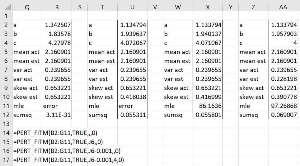
PERT_FITM also supports the approach described in Method of Moments: PERT Distribution of estimating the distribution parameters by solving simultaneous equations. This is done by setting iter = 0 (as for TRIANG_FITM).
Examples are shown in Figure 2. Note that =PERT_FITM(B2:G11,TRUE,,,0) produces the result obtained by solving three equations in three unknowns shown in Figure 1 of Method of Moments: PERT Distribution. As described there, this result produces an excellent fit but violates the rule that a ≤ min.
Figure 2 – PERT_FITM with iter = 0
Examples Workbook
Click here to download the Excel workbook with the examples described on this webpage.
References
Rao, K. S., Viswam, N., Anjaneyulu, G. (2021) Estimation of parameters of Pert distribution by using method of moments
https://www.ijraset.com/fileserve?FID=38239
Wikipedia (2023) PERT distribution
https://en.wikipedia.org/wiki/PERT_distribution

