Objective
We show how to fit data to a 3-parameter Weibull distribution. We do this by using Newton’s method to estimate the three parameters that maximize the log-likelihood function.
Log-likelihood Function
The likelihood function for the sample data x1, …, xn from a 3-parameter Weibull distribution is


![]()
MLE Approach
We now show how to maximize LL using Real Statistics’ MNEWTON3 function.
Example 1: Fit the data in column A of Figure 1 to a 3-parameter Weibull distribution using the MLE approach.
This is the same data used in Example 1 of Method of Moments: Fitting a 3-Parameter Weibull Distribution.
Using initial guesses of ones, the MNEWTON3 function doesn’t arrive at a solution as shown in Figure 1.
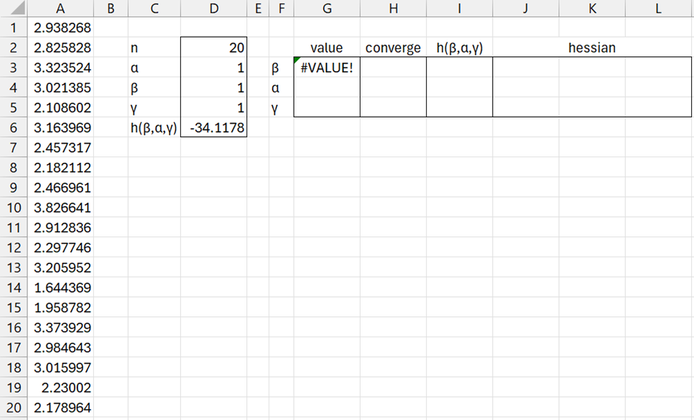
Figure 1 – Initial MLE attempt
Here, cell D6 contains the LL value as calculated by the formula
=D$2*LN(D4)-D$2*D4*LN(D3)+(D4-1)*SUMPRODUCT(LN(A$1:A$20-D5))-SUMPRODUCT((A$1:A$20-D5)^D4)/D3^D4
Note that we use relative addressing for α, β, γ, and absolute addressing for any other variables. Also note that the formula uses the address, D4, for β before the address for α, D3.
Range G3:L5 contains the formula =MNEWTON3(D6,D4,D3,D5).
If we use Solver instead, we will find that Solver would also not converge to a solution. It turns out that our initial guesses need to be fairly close to the optimum values. For example, using the initial guesses shown in range D3:D5 of Figure 2, MNEWTON3 does converge to the solution shown in range G3:G5 with LL = -16.1217 (cell I3).
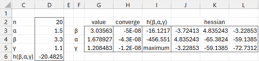
Figure 2 – MLE solution using NEWTON3
The good news is that this time γ takes a value less than the minimum data value of 1.644369 (unlike the situation in Example 1 of Method of Moments: Fitting a 3-Parameter Weibull Distribution).
The situation is fairly similar when using Solver.
Figure 3 shows the actual mean, variance, and skewness values compared to the values for a Weibull distribution with the three fitted parameters.
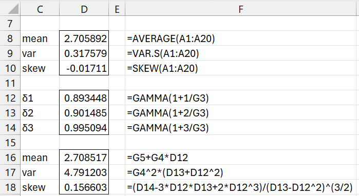
Figure 3 – Judging the fit of the moments
The mean fits pretty well (the value in cell D8 compared to that in cell D16), but the variance and even the skewness are quite far off.
Different Approach
Let’s use try a different approach. Since we used the formula =WEIBULL_INV(RAND(),3,2,1) to construct the sample data in Figure 1, let’s assume that γ = 1, resulting in the revised sample in column B of Figure 4. We now find the MLE fit for the two-parameter Weibull distribution using Real Statistics’ WEIBULL_FIT function, as shown in the rest of Figure 4.
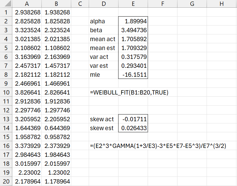
Figure 4 – Two parameter fit
Unsurprisingly, this fit is pretty good. Even the skewness fit is reasonable. The only problem is that in general we don’t know the value of gamma. We do know that it is somewhere between 0 and the smallest sample data value, 1.644369. and so we can repeat the analysis from Figure 4 using various values of gamma between 0 and 1.644369. The results are displayed in Figure 5.
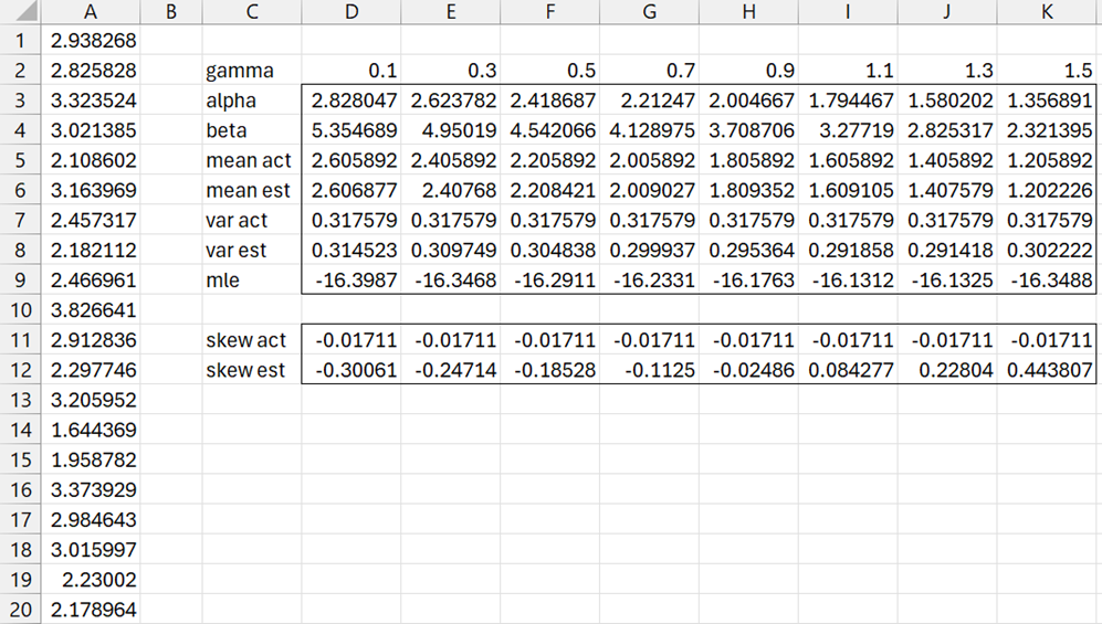
Figure 5 – Finding the best gamma value
E.g. range C3:D9 contains the formula =WEIBULL_FIT($A1:$A20-D2,TRUE), cell D11 contains =SKEW($A1:$A20-D2) and cell D12 contains
=(D3^3*GAMMA(1+3/D4)-3*D6*D8-D6^3)/D8^(3/2).
Of the eight gamma values in Figure 5, γ = 1.3 produces the lowest LL value, namely -16.1312. Thus, we see that parameters in range I2:I4 provide a reasonably good fit. If instead of eight gamma values, we investigate more gamma values, we should expect a little better result.
One can argue that the parameters in columns G or H might even be better since the LL values are only slightly higher than that for column I, but the skewness fit is better. In fact, we can perform the same analysis using the =WEIBULLM_FIT instead of =WEIBULL_FIT to find an optimum method of moments fit instead of an MLE fit.
Worksheet Functions
The Real Statistics Resource Pack provides the following two functions.
WEIBULL3_FIT(R1, lab, iter, witer, bguess) = returns an array with the Weibull distribution parameter values alpha, beta, gamma, actual and estimated mean, variance and skewness, and MLE, based on finding the highest two-parameter MLE fit
WEIBULL3_FITM(R1, lab, iter, witer, bguess) = returns an array with the Weibull distribution parameter values alpha, beta, gamma, actual and estimated skewness, and MLE, based on finding the least difference between the actual and estimated skewness
iter = the number of equally spaced values of gamma evaluated between zero and the smallest value in R1 (default 100). witer = the number of iterations used by WEIBULL_FIT or WEIBULL_FITM when evaluating each gamma value (default 20). Similarly, bguess is the initial guess for beta used by these worksheet functions.
When lab = TRUE (default FALSE), an extra column of labels is appended to the output.
For Example 1, the output from these two functions is shown in Figure 6.
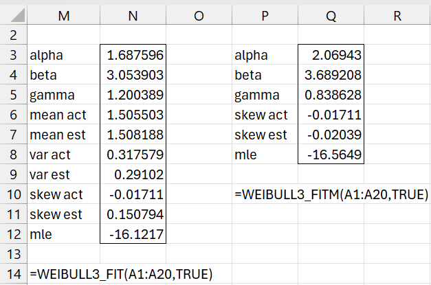
Figure 6 – WEIBULL_FIT and WEIBULL_FITM
Examples Workbook
Click here to download the Excel workbook with the examples described on this webpage.
References
Wikipedia (2021) The Weibull distribution
http://reliawiki.org/index.php/The_Weibull_Distribution
Cousineau, D. (2008) Fitting the three-parameter Weibull distribution: review and evaluation of existing and new methods
http://www.mapageweb.umontreal.ca/cousined/home/others/distrifitting/docs/31_fitweibull_vieee_vproofs.pdf