In Box-Cox Normal Transformation, we describe how to perform a Box-Cox transformation for normality. We now present some optional features.
Review
If all the data are positive, then the usual Box-Cox transformation is
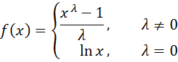
If there are some negative or zero values, then we can use the following modification
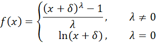
where δ is some parameter such that x + δ > 0 for all x. E.g. δ = γ – min x for some γ > 0.
In Box-Cox Normal Transformation, we use γ = 1.
Hawkins-Weisberg Transformation
When the data contains a non-positive value, the Hawkins-Weisberg version of the Box-Cox transformation often yields less biased results.
This version uses the first version of the Box-Cox transformation, replacing x by h(x) where
![]()
Here, provided γ > 0.
If all the x > 0, then γ is set to 0
Worksheet Functions
Real Statistics Functions: Starting with Rel 9.8, Real Statistics Resource Pack provides the following revised versions of the functions described in Box-Cox Normal Transformation, .
BOXCOX(R1, λ, γ, hw): array function which returns a range containing the Box-Cox transformation of the data in range R1 using the given λ and γ values. If the λ argument is omitted, then the transformation which best normalizes the data in R1 is used, based on maximizing the log-likelihood function (using BOXCOXLambda with the default values of mn, mx, prec, and iter).
BOXCOXLL(R1, λ, γ, hw) = log likelihood function of the Box-Cox transformation of the data in R1 using the given λ and γ values
BOXCOXLambda(R1, mn, nx, iter, prec, γ, hw) = the value of λ that maximizes the log likelihood function of the Box-Cox transformation of the data in R1
When hw = False, then the original version of the Box-Cox transformation, as described above, is used. If R1 contains any non-positive values, then γ – min of the values in R1 is added to all elements in R1.
When hw = True, then the Hawkins-Weisberg version of the transformation is used based on the specified version of gamma.
γ defaults to 1, but is only used if R1 contains non-positive values.
When computing the optimum value of lambda, BOXCOXLambda uses a binary-like search of values of lambda initially between mn (default -3) and mx (default 3). It performs iter (default 100) iterations. A value of lambda less than prec (default .0000001) is considered to be zero. Note, too, that the value of γ is fixed and is not optimized.
Examples
Example 1: Perform a Box-Cox transformation for the data on the left side of Figure 1 using the optimum lambda value when gamma = 1.
The optimum lambda value, shown in cell D3 of Figure 1, is estimated using the formula =BOXCOXLambda(A4:A13). The corresponding Box-Cox transformation, as shown in range D4:D13, is calculated by =BOXCOX(A4:A13, D3) or =BOXCOX(A4:A13). The log-likelihood for this transformation, shown in cell D14, is calculated by =BOXCOXLL(A4:A13, D3).
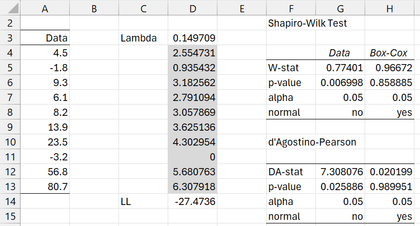
Figure 1 – Box-Cox transformation with non-positive values
You can also calculate the Box-Cox transformed values directly. E.g. to calculate the value in cell D4, you first calculate the minimum data value of -3.2 using the formula =MIN(A4:A13). You then add 1-(-3.2) = 4.2 to the value in cell D4 to obtain 4.5 + 4.2 = 8.2. The resulting value shown in cell D4 is then (8.2 ^ .149709 – 1) / .149709 = 2.554731.
Using the Descriptive Statistics data analysis tool, as shown on the right side of Figure 1, we observe that the original data is not normally distributed, while the transformed data is.
Example 2: Find the Box-Cox transformation for the data in Example 1 when gamma = .5 and 1 for both the original transformation and the Hawkins-Weisberg version.
The result is shown in Figure 2.
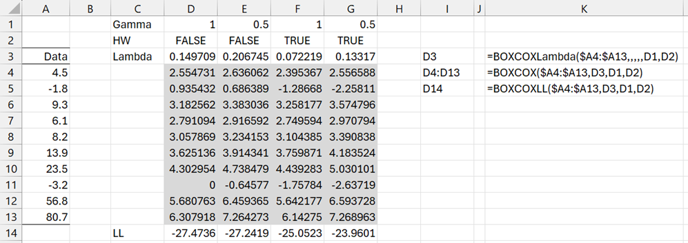
Figure 2 – Various forms of the Box-Cox transformation
Here, we place the formulas shown on the right side of the figure into D3, D4:D13, and D14, then highlight range D3:G14, and press Ctrl-R.
Data Analysis Tool
Real Statistics Analysis Tool: Starting with Rel 9.8, the Real Statistics Resource Pack provides the Box-Cox data analysis tool. This tool enables you to perform Box-Cox transformations for multiple datasets.
To use this tool for Example 1, press Ctrl-m, and select the Box-Cox Transformation option from the Desc tab. Next, fill in the dialog box that appears, as shown in Figure 3.
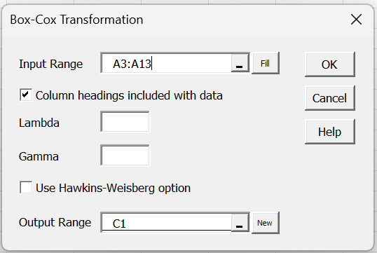
Figure 3 – Dialog Box
Since the Lambda and Gamma fields are left blank, the defaults are used. This means that gamma = 1 and lambda is set to the value that maximizes LL. Since the Hawkins-Weisberg option is unchecked, the original Box-Cox transformation is used.
After clicking on the OK button, the output in columns C and D of Figure 4 appears.
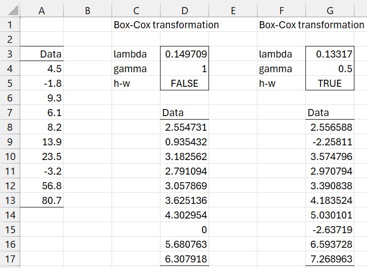
Figure 4 – Box-Cox data analysis
If, in Figure 3, Gamma is set to .5 and the Hawkins-Weisberg option is selected, then the output in columns F and G appears.
Example 3: Perform the Box-Cox transformation for the two datasets on the left side of Figure 5 using the default settings.
This time, you insert A3:B13 in the Input Range of the dialog box in Figure 3. Note that each column in the input is transformed separately.
The output appears on the right side of Figure 5.
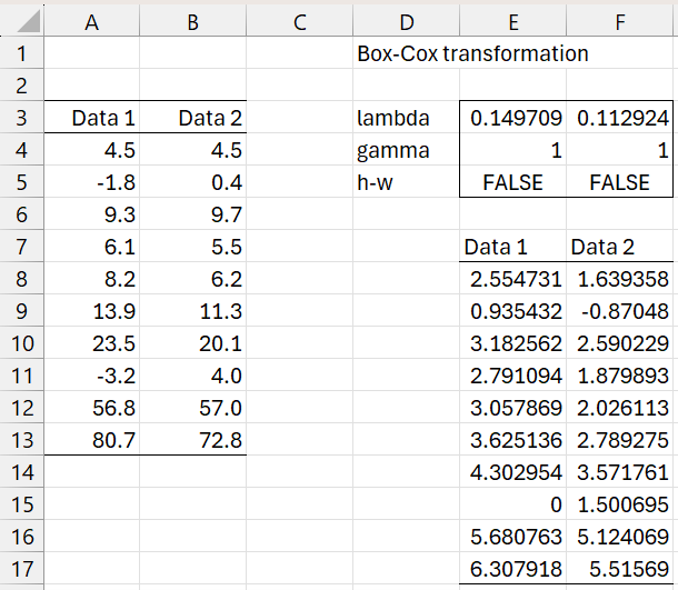
Figure 5 – Box-Cox for multiple datasets
Note that if you change the values in range E3:F5, then the corresponding values in range E8:F17 will change accordingly.
Examples Workbook
Click here to download the Excel workbook with the examples described on this webpage.
Links
References
Hawkins, D. and Weisberg, S. (2017) Combining the Box-Cox power and generalized log transformations to accomodate nonpositive responses in linear and mixed-effects linear models. South African Statistics Journal, 51, 317-328.
https://www.journals.ac.za/index.php/sasj/article/view/5215/3250
Weisberg, S. (2026) bcPower {car}
https://search.r-project.org/CRAN/refmans/car/html/bcPower.html