Introduction
Two-sided Bayesian hypothesis testing is more sensitive to the choice of priors than the one-sided tests (see Bayesian Hypothesis Testing for Normal Data). In fact, choosing non-informative priors tends to produce counter-intuitive results. In particular, even when the alternative hypothesis is true, the posterior test is likely to favor the null hypothesis (Jeffreys–Lindley paradox)
For this reason, instead of non-informative priors, we use weakly informative priors.
One-sample testing
The typical one-sample hypothesis test for data X = x1, …, xn from a normal N(μ, σ2) population (with unknown variance) is based on the following null and alternative hypotheses.
H0: μ = 0
H1: μ ≠ 0
In instead of testing μ, we will test the standard Cohen’s effect size δ = μ/σ. The equivalent null and alternative hypotheses are
H0: δ = 0
H1: δ ≠ 0
Scaled information prior
We use the effect size δ = μ/σ and informative prior δ ∼ N(0, τ1) and non-informative prior σ2 ∝ 1/σ2 or equivalently τ ∝ 1/τ where τ = σ2.
Note that δ ∼ N(0, τ1) is equivalent to μ ∼ N(0, ττ1).
It turns out that the Bayes Factor can be expressed as
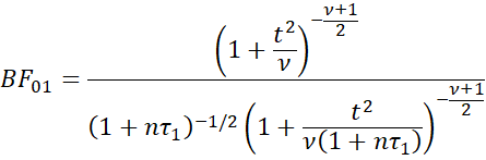
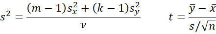
where
![]()
x̄ and s are the usual sample mean and standard deviation.
Setting τ1 too high will result in the Jeffreys–Lindley paradox whereby the test favors the null hypothesis even when the alternative is clearly true. You can set τ1 to a low value, which indicates that the effect size δ is expected to be small since this will indicate that the range of values for δ is expected to be in a narrow band around zero. Recall that the guidelines for δ are: .2 low, .5 medium, and .8 large. Usually, however, you won’t know in advance how small to set τ1.
Setting τ1 = 1 is a reasonable choice since this would mean that the probability that δ is between -1 and +1 is about 68% (one standard deviation from the mean of 0). The model with τ1 = 1 is called the unit information prior.
Setting τ1 = .5 is another popular choice since the probability that δ is between -.8 and +.8 is about 89%. This allows for larger effect sizes but tends to constrain δ to reasonable values.
Note that we usually use notation τ1 = r2. In this case τ1 = 1 or .5 is equivalent to r = 1 or √2/2 ≈ .707.
Scaled JZS prior
Instead of setting the value of τ1 to a fixed value, we can treat it as a hyperparameter to which we need to assign some prior. In particular, setting τ1 ∼ InvChisq(0,1) (see Bayesian Distributions) will provide some additional flexibility, but its value will usually be close to 1.
It turns out that an equivalent approach is to use a Cauchy distribution as a prior for the effect size δ (aka the JZS prior). Thus, we use δ ∼ Cauchy(0, r), i.e. the Cauchy distribution centered around zero and scale factor r with r2 = τ1.
It turns out that the Bayes factor for the JZS prior is
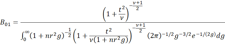
Note that the denominator is an integral, and so we will use Real Statistics’ INTEGRAL worksheet function (see Numerical Integration Function) to compute its value.
The IQR of data from a Cauchy distribution Cauchy(0, r) is approximately twice the value of r. Thus, if r = 1, then the IQR of values will be about 2. Setting r = √2 will increase the IQR by about 40% and setting r = √2/2 ≈ .707 will decrease the IQR by about 30%.
Two independent sample test
The typical two-sample hypothesis test for data X = x1, …, xm from N(μ1, σ2) and Y = y1, …, yk from N(μ2, σ2), where the samples have a common but unknown variance, is based on the following null and alternative hypotheses.
H0: μ1 = μ2
H1: μ1 ≠ μ2
Once again, we use the standard Cohen’s effect size δ = (μ2 – μ1)/σ. The equivalent null and alternative hypotheses are
H0: δ = 0
H1: δ ≠ 0
It turns out that the BF01 based on the scaled information and JZS priors use the same formulas as for the one-sample case, except that now
![]()
Examples
Click here to access numerous Excel examples describing how to perform two-sided hypothesis testing using the Bayesian approach described above.
Real Statistics Support
Click here for a description of Excel worksheet functions and data analysis tools supplied by the Real Statistics Resource Pack that implement the tests described on this webpage.
References
Stack Exchange (2022) Understanding the Jeffreys-Zellner-Siow (JZS) prior in Bayesian t-tests
https://stats.stackexchange.com/questions/570605/understanding-the-jeffreys-zellner-siow-jzs-prior-in-bayesian-t-tests
Rouder, J. N. et al. (2009) Bayesian t tests for accepting and rejecting the null hypothesis
https://www.researchgate.net/publication/24207221_Bayesian_t_test_for_accepting_and_rejecting_the_null_hypothesis
Gonen, M., Lu, Y., Johnson, W. O., Westfall, P. H. (2005) The Bayesian two-sample t-test
https://scispace.com/pdf/the-bayesian-two-sample-t-test-2cf8tnzpmi.pdf
Du, H., Edwards, M. C., Zhang, Z. (2019) Bayes factor in one-sample tests of means with a sensitivity analysis: a discussion of separate prior distributions
https://link.springer.com/content/pdf/10.3758/s13428-019-01262-w.pdf
Faukenberry, T. (2023) Bayesian t-tests
https://www.youtube.com/watch?v=D4RJk3SmhUY