Objective
We describe capabilities provided by the Real Statistics Resource Pack that support hypothesis testing for normally distributed data. These implement the tests described in Bayesian Hypothesis Testing for Normal Data and Bayesian Two-sided Hypothesis Testing.
Worksheet Functions
The Real Statistics Resource Pack provides the following array functions.
BayesT_TEST(t, n1, n2, scale, lab): returns an array with BF01, BF10, P(H0|X), and P(H1|X) for a two-sided weakly informational t test where t = the t-statistic, n1 = size of sample 1, n2 = size of sample 2 (default = 0, which implies this is a one-sample or paired sample test), scale = scale parameter (default √2/2). Here H0: δ = 0 and H1: δ ≠ 0, where δ = μ1 – μ0 for the one-sample test (μ0 = hypothetical mean) or δ = μ2 – μ1 for the two-sample or paired sample test. It is assumed that the population variances in the two independent sample case are equal.
If lab = TRUE (default FALSE), then an extra column of labels is appended to the output.
JZS_TEST(t, n1, n2, scale, lab, iter): exactly as the BayesT_TEST except that the JZS prior is used. iter = the number of iterations used to calculate the integral in the formula for BF01.
For both of these functions, the t-statistic can be calculated using the following non-array worksheet function.
T_STAT(R1, R2, paired) = t statistic
If R2 takes a numeric value, then the t-stat for a one-sample test using the data in R1 is returned, where R2 is the hypothetical mean (default 0). If paired = TRUE (default FALSE), then the t-stat for a paired t-test is returned using the data in R1 and R2; otherwise, the t-stat is for a two independent sample t-test using the data in R1 and R2.
One-sided test functions
The following array function can be used to carry out the one-sided t-test H0: δ < 0 and H1: δ ≥ 0 based on non-informative priors where δ is defined as above.
BayesT0_TEST(t, n, lab): returns an array with Odds01, Odds10, P(H0|X), and P(H1|X) for a one-sided t-test where t = the t-statistic, n = size of sample 1 for the one-sample or paired sample test or the sum of the two sample sizes for a two-sample test. We assume that the population variances for the two independent sample case are equal.
The t-statistic can be calculated using the following non-array worksheet function.
T_STATP(R1, R2, paired) = t statistic based on the population of the variance instead of the sample variance as in T_STAT.
Expanded one-sided functions
The Real Statistics Resource Pack also supports the following functions:
BayesTX_TEST(R1, R2, lab, paired, alpha): returns an array with Odds01, Odds10, P(H0|X), and P(H1|X), (pooled) mean, scale, df, and lower and upper limits of the 1-alpha credible interval.
If R2 takes a numeric value, then this a one-sample test using the data in R1, where R2 is the hypothetical mean (default 0). If paired = TRUE (default FALSE), then a paired t-test is performed using the data in R1 and R2; otherwise, a two independent sample t-test is performed using the data in R1 and R2.
It is assumed that the population variances for the two independent sample case are equal. When they are not equal, especially if they are quite different, then the following function can be used instead.
BayesTS_TEST(R1, R2, lab, iter, alpha): returns an array with Odds01, Odds10, P(H0|X), and P(H1|X), (pooled) mean, and lower and upper limits of the 1-alpha credible interval for the two independent sample t-test based on the data in R1 and R2.
This function uses a simulation with iter iterations (default iter = 10000).
Real Statistics also provides the following counterpart to the BayesT0_TEST function when the variance is known – the var argument in the following description (default var = 1).
BayesZ_TEST(R1, R2, var, lab, paired, alpha): returns an array with Odds01, Odds10, P(H0|X), and P(H1|X), (pooled) mean, scale, df, and lower and upper limits of the 1-alpha credible interval.
Data Analysis Tool
You can also use the Bayesian T Test data analysis tool to perform the various t-tests.
For Example 5 of Bayesian Two-sided Hypothesis Testing, you need to press Ctrl-m and select the Bayesian t Test option from the Bayes tab. Next, fill in the dialog box that appears as shown in Figure 1.
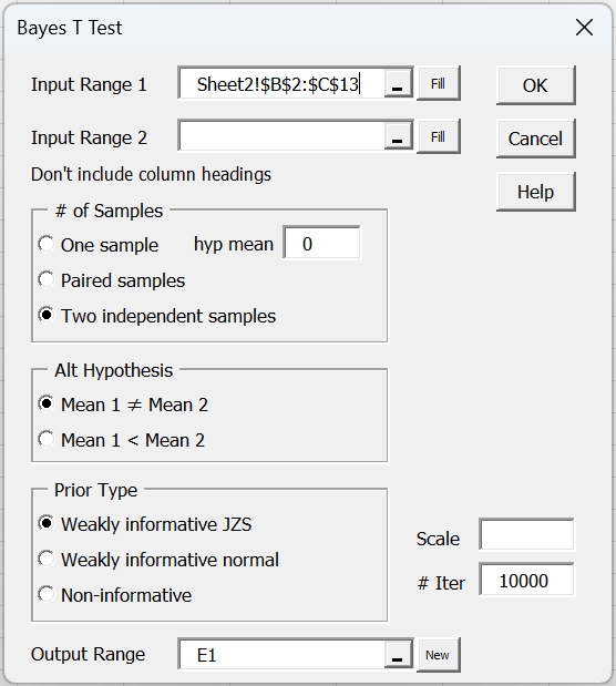
Figure 1 – Bayes t Test dialog box
We plan to perform a two independent sample t-test, and so check this option in the # of Samples section of the dialog box. Next, we enter B2:C13 in Input Range 1 or B2:B13 in Input Range 1 and C2:C13 in Input Range 2. Since we plan to use the weakly informative JZS prior for a two-sided test (H0: mean 1 = mean 2 and H1: mean 1 ≠ mean 2), we retain these default options. Finally, we leave the Scale field blank to select the default √2/2 = .707107 option.
After clicking on the OK button, the output in Figure 2 is displayed (although not all of columns H and I are included in the display).
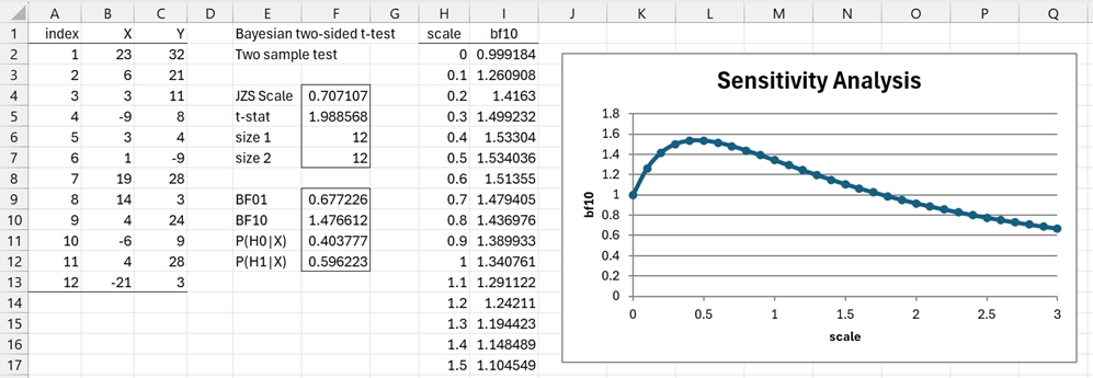
Figure 2 – Two-sided t-test output
Here, cell F5 contains the formula =T_STAT(B2:B13,C2:C13) and range E9:F12 contains the array formula =JZS_TEST(F5,F6,F7,F4,TRUE). Also, cell I2 contains the array formula =INDEX(JZS_TEST(F$5,F$6,F$7,H2),2), and similarly for the other cells in column I.
If instead of choosing the Weakly Informative JZS option in Figure 1, you choose the Weakly Informative Normal option, the output would be similar, but range E9:F12 would contain the array formula =BayesT_TEST(F5,F6,F7,F4,TRUE) with values shown in range B14:B17 of Figure 8 in Bayesian Two-sided Hypothesis Testing. Also, cell I2 would contain the array formula =INDEX(BayesT_TEST(F$5,F$6,F$7,H2),2).
One-sided example
Example 2: This time, we repeat Example 1 only changing the Mean 1 < Mean 2 option in Figure 1. The output is as shown in Figure 3. This time, the results for Mean 1 ≠ Mean 2, Mean 1 < Mean 2, and Mean 1 > Mean 2 are all displayed.
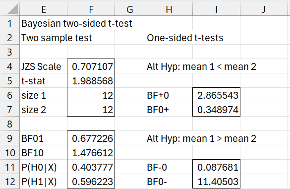
Figure 3 – One-sided t-test output
Columns E and F are the same as those displayed in Figure 2 (for the two-sided test). The results on the right are for the two one-sided tests. Here, we need to use one-sided JZS priors. We estimate these results by using the following approximations (see the Morey and Wagenmakers reference):
BF+0 ≈ (2–p)BF10 if δ ≥ 0
BF-0 ≈ p⋅BF10 if δ ≤ 0
Here p = the frequentist p-value for the two-sided t-test, where δ = (μ2 –μ1)/σ, and so δ > 0 corresponds to the mean 1 < mean 2 case in Figure 3. We obtain the value for BF+0 (comparing H0: μ2 = μ1 with H1: μ2 > μ1) by placing the formula =(2-T.TEST(B2:B13,C2:C13,2,3))*F10 in cell I6. The data analysis tool also calculates BF0+ by placing the formula =1/I6 in cell I7.
Finally, cell I11 contains the formula =T.TEST(B2:B13,C2:C13,2,3)*F10 and cell I12 contains =1/I11.
Another one-sided example
Example 3: This time, we repeat Example 2, selecting the Non-informative prior option in Figure 1. This corresponds to the analysis described in Bayesian Hypothesis Testing for Normal Data.
The output is shown in Figure 4.
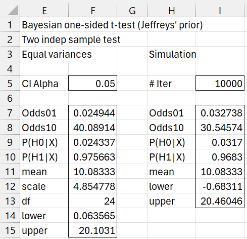
Figure 4 – t-test using Jeffreys’ prior
Here, range E7:F15 contains the array formula =BayesTX_TEST(B2:B13,C2:C13,TRUE,,F5) and range H7:I13 contains the array formula =BayesTS_TEST(B2:B13,C2:C13,TRUE,I5,F5).
If you change the size of the credible interval in cell F5 or the number of simulations in cell I5 (or even any of the cells for the data in B2:C13 of Figure 2), then the output in Figure 4 will change accordingly.
Examples Workbooks
Click here to download the Excel workbook with Bayesian one-sided t-test examples.
Click here to download the Excel workbook with Bayesian two-sided t-test examples.
Finally, click here to download the Excel workbook with examples described on this webpage, plus others for the one-sample and paired sample cases.
References
Reich, B. J., Ghosh, S. K. (2019) Bayesian statistics methods. CRC Press
Lee, P. M. (2012) Bayesian statistics an introduction. 4th Ed. Wiley
https://www.wiley.com/en-us/Bayesian+Statistics%3A+An+Introduction%2C+4th+Edition-p-9781118332573
Jordan, M. (2010) Bayesian modeling and inference. Lecture 1. Course notes
https://people.eecs.berkeley.edu/~jordan/courses/260-spring10/lectures/lecture1.pdf
Gelman, A., Carlin, J. B., Stern, H. S., Dunson, D. B., Vehtari, A., Rubin, D. B. (2014) Bayesian data analysis, 3rd Ed. CRC Press
https://statisticalsupportandresearch.files.wordpress.com/2017/11/bayesian_data_analysis.pdf
Clyde, M. et al. (2022) An introduction to Bayesian thinking
https://statswithr.github.io/book/_main.pdf
Stack Exchange (2022) Understanding the Jeffreys-Zellner-Siow (JZS) prior in Bayesian t-tests
https://stats.stackexchange.com/questions/570605/understanding-the-jeffreys-zellner-siow-jzs-prior-in-bayesian-t-tests
Rouder, J. N. et al. (2009) Bayesian t tests for accepting and rejecting the null hypothesis
https://www.researchgate.net/publication/24207221_Bayesian_t_test_for_accepting_and_rejecting_the_null_hypothesis
Gonen, M., Lu, Y., Johnson, W. O., Westfall, P. H. (2005) The Bayesian two-sample t-test
https://scispace.com/pdf/the-bayesian-two-sample-t-test-2cf8tnzpmi.pdf
Du, H., Edwards, M. C., Zhang, Z. (2019) Bayes factor in one-sample tests of means with a sensitivity analysis: a discussion of separate prior distributions
https://link.springer.com/content/pdf/10.3758/s13428-019-01262-w.pdf
Faukenberry, T. (2023) Bayesian t-tests
https://www.youtube.com/watch?v=D4RJk3SmhUY
Morey, R. D., Wagenmakers, E-J. (2014) Simple relation between Bayesian order-restricted and point-null hypothesis tests
https://www.ejwagenmakers.com/2014/MoreyWagenmakers2014.pdf