Objective
In Creating a Grid using Real Statistics we show how to construct a grid and in Credible Interval and HDI we show how to create a HDI based on the grid. We now show how to use the grid to estimate key statistics (mean, median, etc.) about the population underlying the grid and how to perform hypothesis testing (see Bayesian Hypothesis Testing).
Example
Example 1: Determine the characteristics of the population underlying the posterior distribution described by the grid in Figure 1.
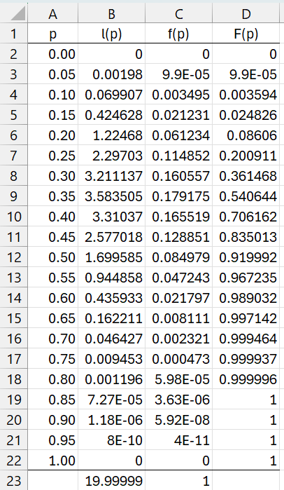
Figure 1 – Bayesian Grid
Column B shows the likelihood values for each of the p values in the grid. The corresponding pdf values are shown in column C and the cdf values in column D. E.g. cell B23 contains formula =SUM(B2:B22), cell C3 contains =B3/B$23, and D3 contains =C3+D2.
First, we note from Figure 1 that f(.4) = .165519 and F(.4) = .706162. To find f(.42) and F(.42) we can use interpolation. To keep things simple, we use linear interpolation. We calculate F(.42) as shown in Figure 2.
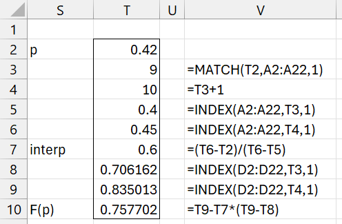
Figure 2 – Using linear interpolation for F(p)
Using the same approach, we find that f(.42) = .150852.
We can also use linear interpolation for the inverse function. E.g. F-1(T10) can be calculated as shown in Figure 3. The good news is that F-1(T10) = .42, as expected.
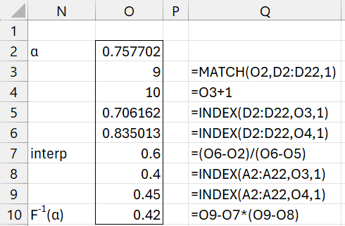
Figure 3 – Using linear interpolation for the inverse
Worksheet Functions
The Real Statistics Resource Pack provides the following functions:
GRID_DIST(x, Rx, Ry, cum) = the pdf f(x) if cum = FALSE based on the grid in Rx and Ry, and the cdf F(x) if cum = TRUE.
GRID_INV(p, Rx, Ry) = the inverse F-1(p) based on the grid in Rx and Ry.
For Example 1, we can calculate the value in cell T10 via the formula
=GRID_DIST(T2,A2:A22,C2:C22,TRUE)
and the value in cell O10 via =GRID_INV(T10,A2:A22,C2:C22). We also calculate f(.42) via =GRID_DIST(T2,A2:A22,C2:C22,TRUE).
Example 1 Continued
Figure 4 displays various characteristics of the posterior distribution for the grid in Figure 1.
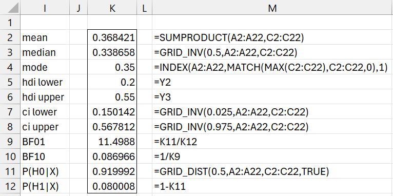
Figure 4 – Grid distribution characteristics
The first three entries in Figure 4 display the mean, median, and mode corresponding to the distribution represented by the grid.
Credible Intervals
Note that the 95% HDI is calculated via the GRID_HDI function shown in Figure 5 (and cells K5 and K6 of Figure 4), as described in Credible Interval and HDI.
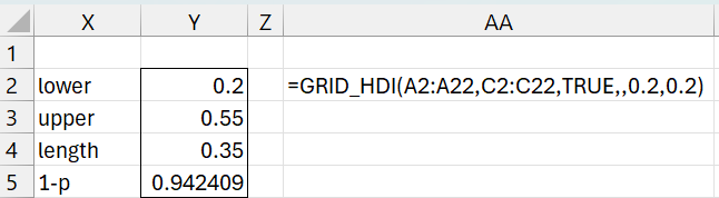
Figure 5 – Grid HDI
Note that we can’t simply use the default .1 value lprec and uprec arguments in =GRID_HDI(A2:A22,C2:C22,TRUE) since with only 21 data points, the no credible interval qualifies as an HDI. By broadening the tolerance from 10% to 20%, we obtain the interval described above. Note that obtained 1-p value of .942409 is too far away from .95 to qualify when lprec = uprec = .1. In fact, since .95 – .05*.1 = .945, 1-p would have to be between .945 and .955. By using lprec = uprec = .2, since .95 – .05*.2 = .94, the value in cell Y5 qualifies since it is between .94 and .96. In fact, even if we use lprec = .16, Y5 would still qualify since .95-.05*.16 = .942 < .942409.
The credible interval shown in range K7:K8 of Figure 4 is the 95% interval with equal tails.
Hypothesis Testing
The values in range I9:K12 are used for hypothesis testing based on the hypotheses
H0: p < .5
H1: p ≥ .5
We see that the null hypothesis is about 11.5 times more likely than the alternative hypothesis (assuming that the priors were equally likely) as explained in Bayesian Hypothesis Testing.
Worksheet Function
The Real Statistics Resource Pack provides the following worksheet function:
GridDesc(Rx, Ry, lab, hyp, alpha, lprec, uprec): returns an array like K2:K12 in Figure 4 based on the grid in Rx and Ry.
1-alpha specifies the equal-tailed credible interval and HDI (default for alpha is .05). lprec and uprec are as described for GRID_HDI. hyp is the value used for hypothesis testing (default 0). For Example 1, we use hyp = .5. As usual, if lab = TRUE (default FALSE) a column of labels is appended to the output.
For Example 1, we could have obtained the output shown in range K2:K12 of Figure 4 by using the formula
=GridDesc(A2:A22,C2:C22,,0.5,0.05,0.2,0.2)
Finer analysis
It turns out that data used in Figure 1 was derived from a beta distribution. In particular, cell B2 contains the formula =BETA.DIST(A2,7,12,FALSE), and range B2:B22 was highlighted and Ctrl-D was pressed. Thus, the grid represents a course characterization of a beta distribution with parameters alpha = 7 and beta = 12. As described in Bayesian Characterization of a Beta Distribution, we can use the array formula =BayesBeta(7,12,TRUE) to create the output shown in Figure 6.
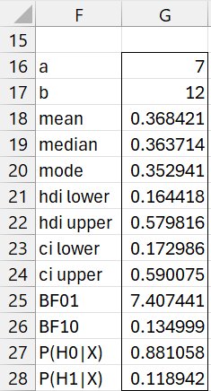
Figure 6 – Beta distribution characteristics
We see that many of the entries in Figure 4 are reasonable approximations of the corresponding entry in Figure 6. We can improve the accuracy by adding more data to that shown in Figure 1 by spline interpolation. This results in a grid with 201 entries instead of 21, as shown in Figure 7 (only the first and last few entries are displayed).
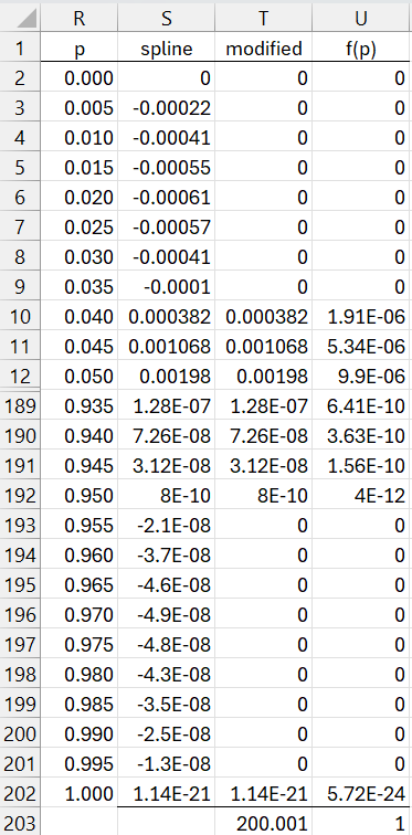
Figure 7 – Spline expansion
The figure is constructed by inserting 0 in cell R2, the formula =R2+.005 in cell R3, highlighting range R3:R202, and pressing Ctrl-D. Next, we insert the array formula =SPLINE(R2:R202,A2:A22,B2:B22) in range S2:S202. We now replace all negative entries in column S by zero, as shown in column T. Finally, we divide all the entries in column T by the sum of these entries (as shown in cell T203) to create the finer representation of the pdf as shown in column U.
We now create a revised version of Figure 4 using the finer grid from Figure 7. This is done by using the array formula =GridDesc(R2:R202,U2:U202,TRUE,0.5). The output is shown in Figure 8.
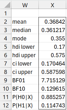
Figure 8 – Improved results
This output is a little closer to that shown in Figure 6.
Charts of the data from Figures 1 and 7 are shown in Figure 9.
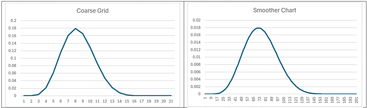
Figure 9 – More data, smoother chart
Worksheet Function
The Real Statistics Resource Pack provides a simpler way to obtain the results shown in Figure 7.
GridSpline(Rx, Ry, rate): returns a two-column array with an expansion to the grid defined by Rx and Ry. The first column of the output contains the x values while the second column contains the corresponding y values where each value in the original grid except the last is expanded to rate (default 10) number of values using spline interpolation.
The output from =GridSpline(A2:A22,C2:C22) consists of a two-column array with the data in R2:R202 and U2:U202. Actually, you can obtain the same results from the array formula =GridSpline(A2:A22,B2:B22).
Examples Workbook
Click here to download the Excel workbook with the examples described on this webpage.
References
Kruschke, J. K. (2015) Doing Bayesian data analysis. 2nd Ed. Elsevier
https://sites.google.com/site/doingbayesiandataanalysis/
Chechile, R. A., Barch, D. H. Jr. (2025) Distribution-free Bayesian analyses with the DFBA statistical package
https://link.springer.com/article/10.3758/s13428-025-02605-6
Chechile, R. A. (2018) A Bayesian analysis for the Wilcoxon signed-rank statistic. Communications in Statistics – Theory and Methods
https://doi.org/10.1080/03610926.2017.1388402