Example
Example 1: Repeat Example 1 of Two Binomial Samples Beta Prior using the Metropolis algorithm described in Random Walk Metropolis Algorithm.
We proceed as in Example 1 of Random Walk Metropolis Algorithm, except that now we use a bivariate normal distribution as our proposal distribution. In particular, we use a bivariate normal distribution with standard deviation .1 for both dimensions and 0 correlation. We can use the formula =BNORMDIST(x1,x2,m1,m2,s1,s2,r,TRUE) to compute the value of the bivariate normal distribution. Since the correlation r is zero, we can use the following formula instead:
=NORM.DIST(x1,m1,s1,TRUE)*NORM.DIST(x2,m2,s2,TRUE).
Results
The results, using a very small sample of 500 elements, is shown in Figure 1. The mean p = .850629 and q = .424495 is pretty close to the theoretical mean values p = α/(α+β) and q = γ/(γ+δ) of the posterior beta distributions, as shown in cells J15 and J16.
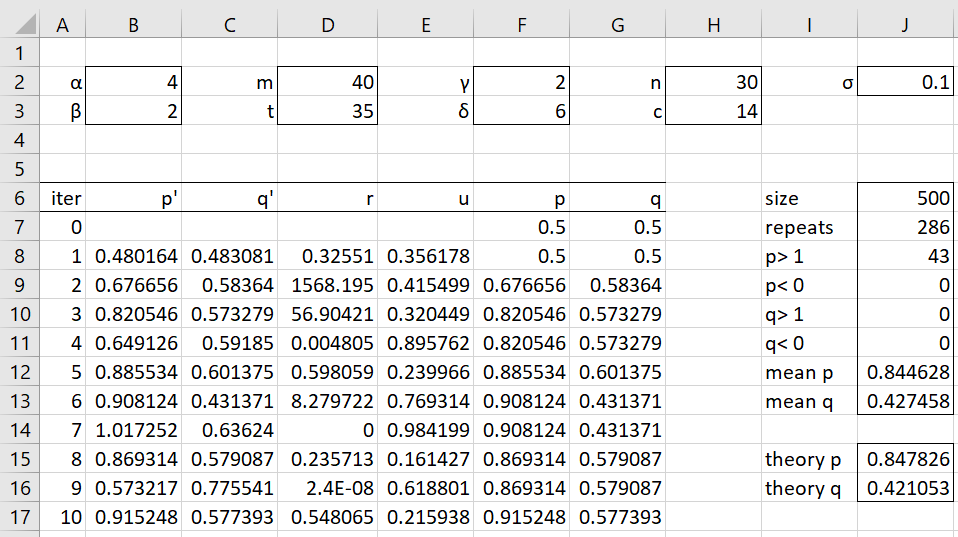
Figure 1 – Metropolis algorithm
Key formulas from Figure 1 are shown in Figure 2.
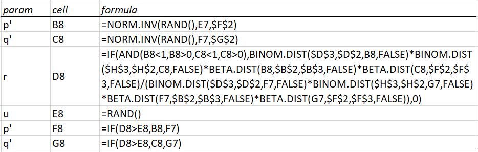
Figure 2 – Key formulas from Figure 1
Analysis
If we look at the 500 sample values of p–q (see Figure 3, which only shows the first 5 values), we see that except for the first value, for all the others p > q, which again gives us a high degree of confidence that the drug is effective. Here, cell O7 contains the formula =COUNTIF(L8:L507,”>0″)/$J$6.
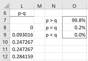
Figure 3 – p minus q
Examples Workbook
Click here to download the Excel workbook with the examples described on this webpage.
References
Gelman, A., Carlin, J. B., Stern, H. S., Dunson, D. B., Vehtari, A., Rubin, D. B. (2014) Bayesian data analysis, 3rd Ed. CRC Press
https://statisticalsupportandresearch.files.wordpress.com/2017/11/bayesian_data_analysis.pdf
Lee, P. M. (2012) Bayesian statistics an introduction. 4th Ed. Wiley
https://www.wiley.com/en-us/Bayesian+Statistics%3A+An+Introduction%2C+4th+Edition-p-9781118332573