Example
Example 1: Repeat Example 1 of Two Binomial Samples Beta Prior using the grid approach described in Bayesian Grid Approximation. Also estimate the 95% high density region.
We first create two grids, one for p and one for q (where only the first half of each is displayed), as we did in Figure 1 of Bayesian Grid Approximation. The result is shown in Figure 1.
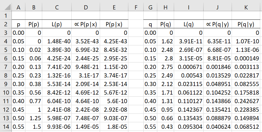
Figure 1 – Grids for p and q
Each of these grids contains values in .05 increments from 0 to .95 (row 3 to row 22). Figure 2 shows the grid for (p, q), which consists of 20 × 20 = 400 rows, only the last 17 rows of which are visible.
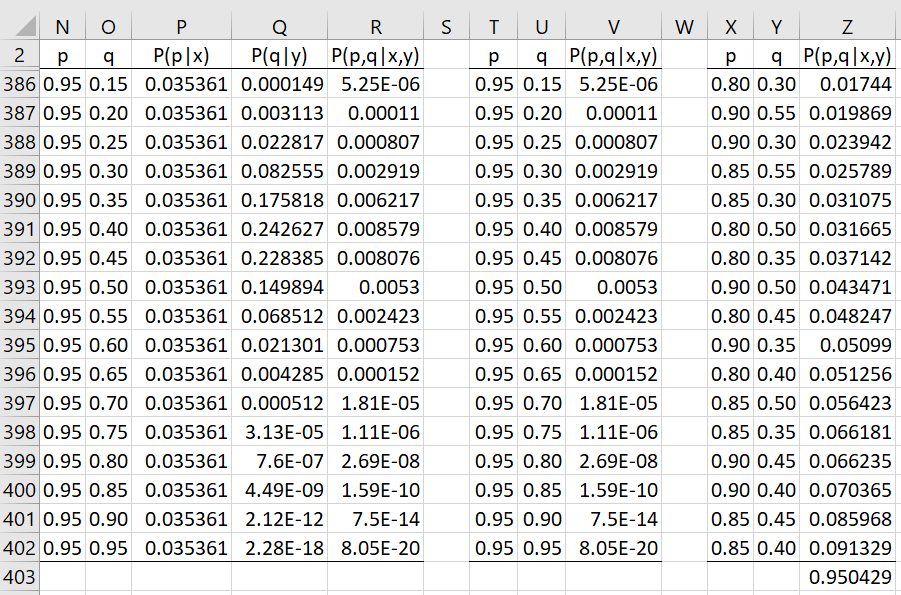
Figure 2 – Grid for (p, q)
Columns N and O contain all pairs from columns A and G, while columns P and Q contain the corresponding values from columns E and K. The elements in column R contain the product of the corresponding elements from columns P and Q. Columns T, U and V contain copies of the elements from columns N, O and R, and represents an approximation of the posterior distribution.
Finally, range X2:Z402 contains the data in columns T, U and V in sorted order based on the sort key in column V. We accomplish this by placing the array formula =QSORTRows(T2:V402,3,TRUE,TRUE) in range X2:Z402.
95% HDI
The values in column Z sum up to one as expected, but the sum of the highest values, namely those from cell Z372 to Z402 sum up to approximately .95, and so represent a 95% high density region. This is shown in cell Z403, with value .950429 as calculated by the formula =SUM(Z372:Z402). We can plot the 31 pairs (p, q) in this range, i.e. Z372:Z402, using a scatter chart as shown in Figure 3.
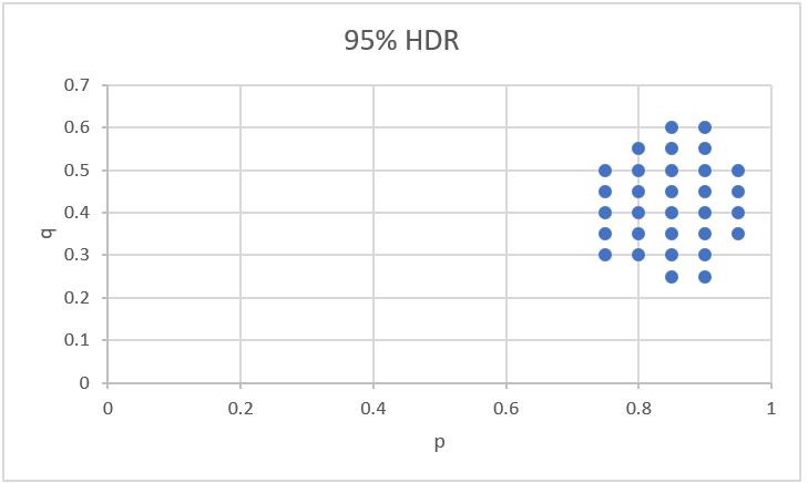
Figure 3 – High Density Region
It turns out that p > q for all the pairs in the 95% HDR (which is partially visible also in columns X and Y of Figure 2). This clearly supports the hypothesis that the treatment is effective, i.e. the proportion of people cured in the treatment group is higher than the people cured in the control group. In fact, the probability that p > q is 99.997%, as calculated by the worksheet formula =SUM(IF(X3:X402>Y3:Y402,Z3:Z402,0)).
Credible ellipse
Note that the two-dimensional equivalent of a credible interval is a credible ellipse. The region in Figure 3 looks similar to an ellipse. To find a 95% credible ellipse, we would need to find values (a, b) and (c, d) such that the posterior (p, q) values lie inside the ellipse, i.e. a ≤ p ≤ b and c ≤ q ≤ d, and the sum of the P(p,q|x,y) values for all such (p, q) is .95. We see that the 95% high density ellipse is the one with the smallest area. Since the area of an ellipse is π(b–a)(d–c), our goal is to minimize (b–a)(d–c) subject to the previous constraints.
Since the 95% HDR uses .70 ≤ p ≤ .95 and .25 ≤ q ≤ .60, we experiment with various ellipses in Figure 4 near these values.
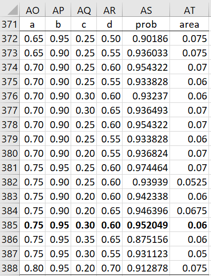
Figure 4 – High density ellipse
We see that the ellipse defined by .75 ≤ p ≤ .95 and .30 ≤ q ≤ .60 is the one with the smallest area that is pretty close to .95. Note that p < q for all the pairs in this ellipse.
Examples Workbook
Click here to download the Excel workbook with the examples described on this webpage.
References
Kruschke, J. K. (2015) Doing Bayesian data analysis. 2nd Ed. Elsevier
https://sites.google.com/site/doingbayesiandataanalysis/
Gelman, A., Carlin, J. B., Stern, H. S., Dunson, D. B., Vehtari, A., Rubin, D. B. (2014) Bayesian data analysis, 3rd Ed. CRC Press
https://statisticalsupportandresearch.files.wordpress.com/2017/11/bayesian_data_analysis.pdf
Marin, J-M and Robert, C. R. (2014) Bayesian essentials with R. 2nd Ed. Springer
https://www.springer.com/gp/book/9781461486862
Jordan, M. (2010) Bayesian modeling and inference. Course notes
https://people.eecs.berkeley.edu/~jordan/courses/260-spring10/lectures/index.html
Lee, P. M. (2012) Bayesian statistics an introduction. 4th Ed. Wiley
https://www.wiley.com/en-us/Bayesian+Statistics%3A+An+Introduction%2C+4th+Edition-p-9781118332573