Objective
Just as we have provided for distributions represented by a grid (see Bayesian Analysis using Grids), we can create a Bayesian characterization of a population distribution. In particular, we show how to do this for a beta distribution.
Example
Example 1: Provide a description of the beta distribution with parameters alpha = 7 and beta = 17 useful for further Bayesian analysis.
This is shown on the left side of Figure 1.
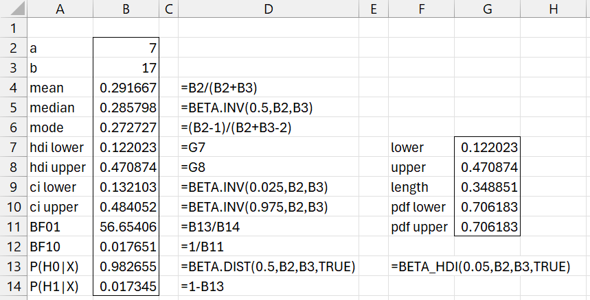
Figure 1 – Bayesian characterization of Bet(7,17)
The 95% HDI for the beta distribution (cells B7:B8) are calculated using the BETA_HDI as described in High Density Interval and shown in range F7:G11.
The 95% credible interval shown in B9:B10 is the equal-tailed CI.
The hypothesis testing is for the hypotheses
H0: p < .5
H1: p ≥ .5
We see that the null hypothesis is more than 56 times more likely than the alternative hypothesis (assuming that the priors were equally likely) as explained in Bayesian Binomial Hypothesis Testing.
Worksheet Function
The Real Statistics Resource Pack provides the following function:
BayesBeta(a, b, lab, alpha, hyp): returns an array like B2:B14 in Figure 1 for a beta distribution with parameters a and b, and hypothetical test value hyp (default .5).
1-alpha specifies the equal-tailed credible interval and HDI (default for alpha is .05). If lab = TRUE (default FALSE) a column of labels is appended to the output.
For Example 1, we could have obtained the output shown in range A2:B14 of Figure 1 by using the formula =BayesBeta(7, 17, TRUE).
Examples Workbook
Click here to download the Excel workbook with the examples described on this webpage.
References
Kruschke, J. K. (2015) Doing Bayesian data analysis. 2nd Ed. Elsevier
https://sites.google.com/site/doingbayesiandataanalysis/
Chechile, R. A., Barch, D. H. Jr. (2025) Distribution-free Bayesian analyses with the DFBA statistical package
https://link.springer.com/article/10.3758/s13428-025-02605-6