Objectives
On this webpage, we provide an example of how to perform the Bayesian Mann-Whitney test in Excel, using both the small and large sample methods. These are described in Bayesian Mann-Whitney Test.
We also describe some Real Statistics capabilities to support this test.
Small Sample Example
Example 1: Use the Bayesian Mann-Whitney test to determine whether Y is stochastically dominant over X (the alternative hypothesis) based on the data in columns A and B of Figure 1. This is done by testing whether θX < .5 (where θX is as defined in Bayesian Mann-Whitney Test). Y is stochastically dominant over X if when you randomly pick elements x0 and y0 from the populations from which X and Y were drawn, then the probability that y0 > x0 is greater than 50%.
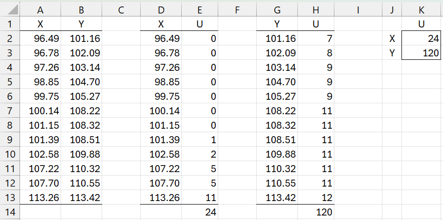
Figure 1 – Data for Mann-Whitney Test
The first thing we do is calculate UX and UY. We see that UX = 24 (cell E14), as calculated by the formula =SUM(E2:E13). The values in column E are determined by inserting the formula =COUNTIF(B$2:B$13,”<“&A2) in cell E2, highlighting E2:E13, and pressing Ctrl-D. UY in cell H14 is calculated in the same way by reversing the roles of X and Y. Since there are no ties UX + UY = mn where m and n are the sizes of the two samples.
Creating a grid
We now perform the Mann-Whitney test as described in Figure 2 (the middle rows are not displayed). We start by inserting .0025 in cell D2, the formula = D2+.005 in cell D3, highlighting range D3:D201, and pressing Ctrl-D to fill in column D. Next, we insert the formula =BayesMW1(A$16,B$16,A$19,D2) in cell E2, highlight range E2:E201, and press Ctrl-D to fill in column E. We use the Real Statistics function BayesMW1 to perform the Monte Carlo sampling with 30,000 iterations for each of the 200 values of theta, as described in Bayesian Mann-Whitney Test. See below for a description of this worksheet function.
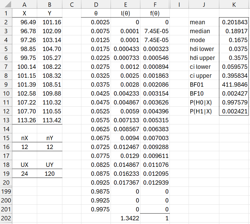
Figure 2 – Bayesian Mann-Whitney Test
We next sum the likelihood values in column E by placing the formula =SUM(E2:E201) in cell E202. The 200 pdf values are now calculated by placing the formula =E2/E$202 in cell F2, highlighting range F2:F201, and pressing Ctrl-D.
Output
Finally, we create a description of the grid produced in columns D and F by placing the array formula =GridDesc(D2:D201,F2:F201,TRUE,0.5) in range J2:K12.
We conclude that there is decisive support for the alternative hypothesis that Y stochastically dominates X. In fact, the probability that the alternative hypothesis holds is 99.76% with a Bayes Factor BF10 of 412.
Large Sample Example
Example 2: Repeat Example 1 using a large sample approximation.
We start by calculating UX, UY, nX, and nY. These are copied into cells J2, J3, J6, and J7 of Figure 3.
We next carry out the approach described above, and shown in Figure 3.
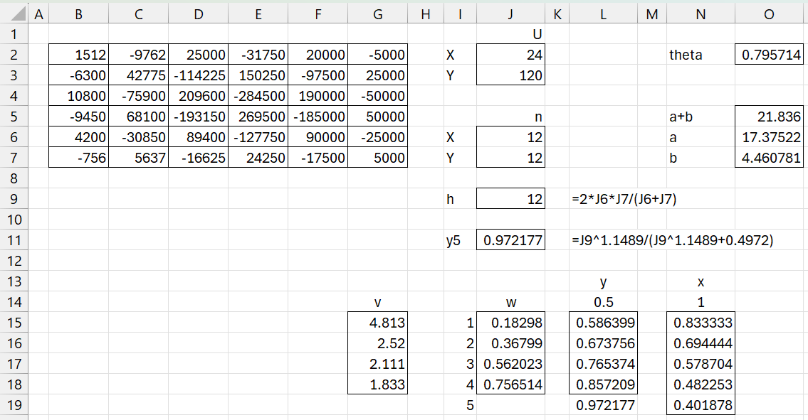
Figure 3 – Start of MW large sample approximation
The L, v, and w values are constants as well as the values in cells L14 and N14. Cell L19 contains the formula =J11. Cell L15 contains the formula =J$11*J15+0.5*(1-J15), cell N15 contains the formula =MAX(J2:J3)/SUM(J2:J3), and cell N16 contains =N$15*N15. The remaining cells are filled in by highlighting L15:L18 and pressing Ctrl-D and highlighting N16:N19 and pressing Ctrl-D.
Cell O2 contains =MMULT(TRANSPOSE(L14:L19),MMULT(B2:G7,N14:N19))/6 and cell O5 contains =J9*(1.028+0.75*N15)+2. Cells O6 and O7 contain =O2*O5 and =O5-O6.
Finally, we use the array formula =BayesBeta(O6,O7,TRUE) to obtain the results shown in Figure 4. We see that the probability that Y dominates X is 99.8% with a Bayes Factor BF10 = 573.455.
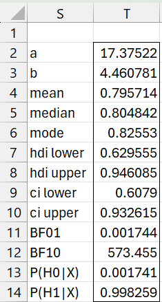
Figure 4 – Large sample MW analysis
Even though the sample sizes are below the usual recommendation for the large sample approach, the results shown in Figure 4 are reasonably similar to those obtained in Figure 2.
Worksheet Functions
The Real Statistics Resource Pack provides the following worksheet functions. Rx and Ry are column arrays containing numeric data.
BayesMWU(Rx, Ry): returns UX
BayesMWX(Rx, Ry, iter): returns a column array with 200 entries corresponding to values of theta from .0025 to .9975 in .005 increments. Each entry contains the pdf value based on the iter-many Monte Carlo sample pairs that produce a UX value equal to the UX value for the original sample Rx and Ry. iter defaults to 30000.
BayesMWSm(Rx, Ry, lab, iter, alpha, lprec, uprec): returns an array with nX, nY, UX, UY, mean, median, mode, 1-alpha HDI lower/upper, 1-alpha equal-tailed CI lower/upper, and hypothesis test BF01, BF10, P(H0|X,Y) and P(H1|X,Y) based on the null hypothesis θX < .5 (equivalent to X stochastically dominates Y). The output is based on a grid created using 200 phi values starting from .0025 in increments of .005 based where each grid entry is calculated using iter-many Monte Carlo samples (default iter = 30000). lprec and uprec are defined as for GRID_HDI.
BayesMWLg(Rx, Ry, lab, a, b, alpha): returns an array with nX, nY, UX, UY, the posterior Beta parameters, mean, median, mode, 1-alpha HDI lower/upper, 1-alpha equal-tailed CI lower/upper, and hypothesis test BF01, BF10, P(H0|X,Y) and P(H1|X,Y) for a Bayesian Mann-Whitney test based on the null hypothesis θX < .5 (equivalent to X stochastically dominates Y). The output is based on a Beta distribution approximation using a Beta prior with parameters a (default 1) and b (default 1).
More worksheet functions
The Real Statistics Resource Pack also provides the following non-array worksheet function:
BayesMW1(n1, n2, u1, theta, iter) = the proportion of the iter-many Monte Carlo sample pairs of size n1 and n2 (default of iter = 30000) produce a U1 value equal to u1 based on the specified theta value. This value serves as the likelihood estimate for the specified value of theta.
We also have the following array function for a Mann-Whitney test based on any two independent samples of sizes n1, n2 and U values u1, u2.
BayesMW1X(n1, n2, u1, iter): returns a column array with 200 entries corresponding to values of theta from .0025 to .9975 in .005 increments. Each entry contains the pdf value based on the iter-many Monte Carlo sample pairs that produce a U1 value equal to u1 based on samples of size n1 and n2. iter defaults to 30000.
BayesMW1Sm(n1, n2, u1, lab, iter, alpha, lprec, uprec): equivalent to BayesMWSm for any arrays R1 and R2 which have n1 and n2 entries respectively and has a U1 value equal to u1.
BayesMW1Lg(n1, n2, u1, u2, lab, a, b, alpha): returns an array with the posterior Beta parameters, mean, median, mode, 1-alpha HDI lower/upper, 1-alpha equal-tailed CI lower/upper, and hypothesis test BF01, BF10, P(H0|X,Y) and P(H1|X,Y) for a Bayesian Mann-Whitney test based on the null hypothesis θ1 < .5. The output is based on a Beta distribution approximation using a Beta prior with parameters a (default 1) and b (default 1).
Examples
The values in cells K2 and K3 of Figure 1 can be produced using the formulas =BayesMWU(A2:A13, B2:B13) and =BayesMWU(B2:B13, A2:A13).
You can produce the values in range F2:F201 of Figure 2 by the formula =BayesMWX(A2:A13, B2:B13) or =BayesMW1X(A16, B16, A19). The values in range J2:K12 of that figure can be produced by the formula =BayesMW1Sm(A16, B16, A19, TRUE). The formula =BayesMWX(A2:A13, B2:B13, TRUE) would produce the same output preceded by the nX, nY, UX, UY values of 12, 12, 24, and 120.
You can use the formula =BayesMW1Lg(12, 12, 24, 120, TRUE) to produce the output in Figure 4.
Data Analysis Tool
Example 3: Repeat Example 2 using the Real Statistics Bayesian Non-parametric Tests data analysis tool employing the large sample approach.
Press Ctrl-m and select the Bayesian Non-parametric Tests option from the Bayes tab. Next, fill in the dialog box that appears as shown in Figure 5.
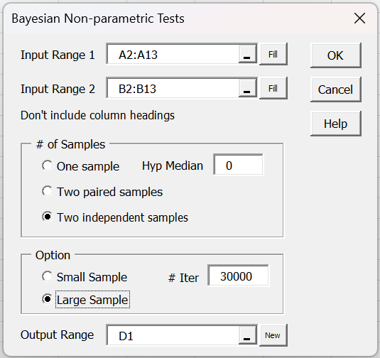
Figure 5 – Bayesian Non-parametric Tests dialog box
After clicking on the OK button, the output shown in Figure 6 appears.
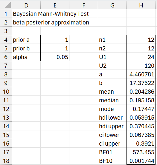
Figure 6 – Bayesian MW Test output
Note that range G4:H18 contains the array formula
=BayesMWLg(A2:A13,B2:B13,TRUE,E4,E5,E6)
where A2:A13 and B2:B13 are as displayed in Figure 1.
Examples Workbooks
Click here to download the Excel workbook with the examples described on this webpage.
Click here for another workbook with additional examples. These workbooks may take a little time to open.
References
Kruschke, J. K. (2015) Doing Bayesian data analysis. 2nd Ed. Elsevier
https://sites.google.com/site/doingbayesiandataanalysis/
Chechile, R. A., Barch, D. H. Jr. (2025) Distribution-free Bayesian analyses with the DFBA statistical package
https://link.springer.com/article/10.3758/s13428-025-02605-6
Chechile, R. A. (2019) A Bayesian analysis for the Mann-Whitney statistic
https://doi.org/10.1080/03610926.2018.1549247