Bayesian Mann-Whitney Test

Objective

Describes the Bayesian version of the non-parametric Mann-Whitney Test. This test is typically used when the assumptions for the two independent sample t-test is not met.

Basic Concepts

Suppose that you have two independent samples X = x₁, …, x_m and Y = y₁, …, y_n, and want to test the hypotheses

H₀: μ_X > μ_Y

H₁: μ_X ≤ μ_Y

We define

We next define the population parameters

Since θ_Y = 1 – θ_X, we only need to consider θ_X. If X is stochastically dominant then θ_X > .5, while if θ_X < .5 then Y is stochastically dominant.

Small Sample Approach

The test consists of performing Monte Carlo sampling for each of 200 discrete values of θ_X ranging from .025 to.9975 in increments of .005. We will call these θ_i where θ_i = .0025 + .005(i–1) for i = 1 to 200.

For each of the 200 values of θ_i, we create a large number of samples (default iter = 30000) of size m from X and of size n from Y. This is done using a little trick. Each Y sample consists of n random values from the exponential distribution f(y) = kexp(-ky) with k = 1, while each X sample consists of m random values from the exponential distribution with k = (1 – θ_i)/θ_i. For each pair of samples, we calculate the value of U_X and see whether it matches the U_X value of the original sample. The proportion of matches is an estimate of the likelihood function P(U_X|θ_i).

The prior for θ_i assumes equal likelihood, namely P(θ_i) = 1/200.

Using Bayes Theorem, it follows that

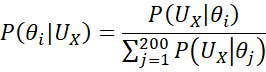
For any θ_i  value, we draw iter many pairs of samples from distributions with this θ_X value. We then count what proportion of the sample pairs have the same U_X values as our original sample. This proportion is the likelihood P(U_X|θ_X).

Large Sample Approximation

Let h = harmonic mean of m and n = 2mn/(m+n). If h > 20 then we can use the following beta distribution approximation.

Define the beta distribution parameters as

a = θ[h(1.028 + .75u) + 2)]

b = (1–θ)[h(1.028 + .75u) + 2)]

where

Here θ is a large sample approximation for θ_X. Obviously, θ = a/(a+b), as expected for the mean of a beta distribution.

We now show how to estimate θ. First, we define x

and X = (1, x, x², x³, x⁴, x⁵). Note that x ≥ .5.

Next, define Y = (.5, y₁, y₂, y₃, y₄, y₅) where

For i = 1, 2, 3, 4 define

where

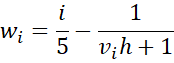
with V = (4.813, 2.520, 2.111, 1.833).

We now define the 6 × 6 matrix L

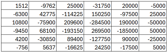
Then our estimate for y (and so θ) is equal to the following matrix multiplication value

Finally, our estimate θ of θ_X is

The above estimates for the posterior beta parameters a and b are based on a uniform prior. For a beta prior Bet(a₀, b₀), the posterior beta distribution is Bet(a+a₀–1, b+b₀–1) where a and b are as described above.

Examples and Excel Support

Click here for examples of how to carry out the Bayesian Mann-Whitney Test in Excel. Also includes a description of various worksheet functions in support of the Bayesian Mann-Whitney Test, as well as an Excel-based data analysis tool.

References

Kruschke, J. K. (2015) Doing Bayesian data analysis. 2nd Ed. Elsevier
https://sites.google.com/site/doingbayesiandataanalysis/

Chechile, R. A., Barch, D. H. Jr. (2025) Distribution-free Bayesian analyses with the DFBA statistical package
https://link.springer.com/article/10.3758/s13428-025-02605-6

Chechile, R. A. (2019) A Bayesian analysis for the Mann-Whitney statistic
https://doi.org/10.1080/03610926.2018.1549247