GMM Example

Objective

We now show how to carry out the GMM procedure described in Univariate GMM. in Excel.

Example

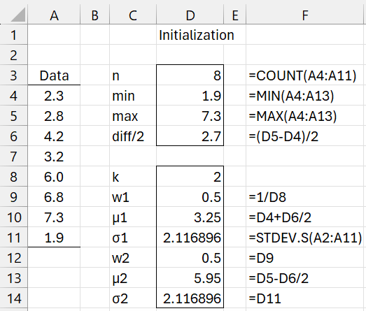
Example 1: Determine the GMM parameters for a two cluster fit of the data in range A4:A11 of Figure 1.

Figure 1 – Initialization

Initialization

There are a number of approaches for initializing the GMM parameters, including using K-means clustering. Instead, we will choose the following approach where the # of clusters is k, the smallest and largest elements in the sample are mn and mx, and d = (mx-mn)/(k-1):

• Estimate w_j by 1/k for each component
• Set μ₁ = mn + d/2 and μ_j = μ_j-1 + d for all j = 2, …, k
• Set σ_j to the standard deviation of the sample for all j

This is the approach used in Figure 1.

EM Algorithm

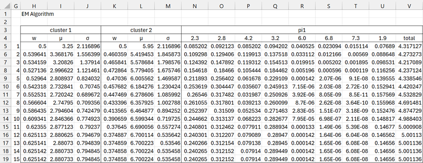
We now perform 15 iterations of the EM algorithm as shown in Figures 2 and 3.

Figure 2 – EM algorithm (part 1)

Range H5:M5 of Figure 2 contains the initial parameter values taken from Figure 1.  The values in range N5:U4 divided by the value in V5 produce the E step-1 values for p₁₁, …, p₈₁.

Figure 3 – EM algorithm (part 2)

The values in range W5:AD4 divided by the value in AM5 produce the E step-1 values for p₁₂, …, p₈₂.

The updated M step values are shown in range H6:M6 of Figure 2.

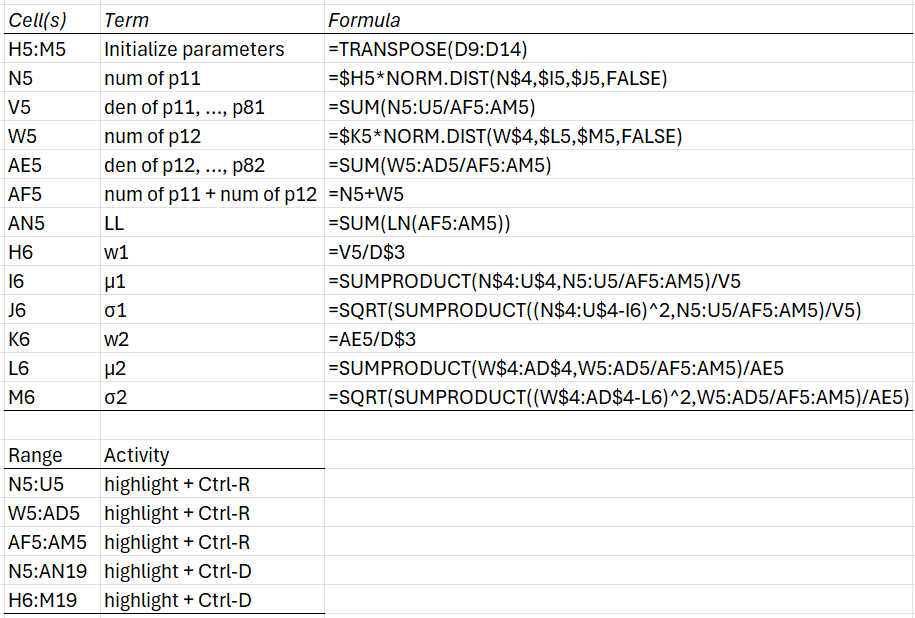
To obtain the spreadsheet shown in Figures 2 and 3, fill in the formulas shown on the upper part of Figure 4. Next, highlight the various ranges listed in the lower part of the figure and press Ctrl-R or Ctrl-D as indicated.

Figure 4 – EM algorithm details

We see that all the values in rows 18 and 19 are equal, indicating that convergence was reached after 14 steps. In fact, LL convergence was reached after 12 steps (comparing cell AN16 with AN17).

In conclusion, the GMM algorithm estimates that the two subpopulations (or components or clusters) have distributions N(2.88, 0.794²) and N(6.70, 0.535²).

Cluster Assignment

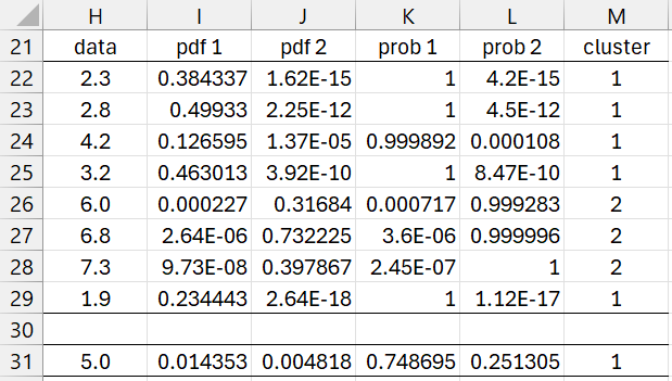
We now determine which subpopulation each of the eight data elements belongs to. This is shown in Figure 5.

Figure 5 – Cluster probabilities

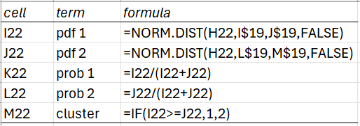
The formulas used for the first data element are shown in Figure 6.

Figure 6 – Formulas from Figure 5

For each data element (shown in column H of Figure 5), we calculate the pdf value for that element for each of the two subpopulations. E.g. the pdf for 6.0 in cluster 1 is .000227, while the pdf for cluster 2 is .31684. Clearly it is more likely that 6.0 is in cluster 2. In fact the probability that 6.0 is in cluster 2 is 99.9283%.

We see that 5 of the 8 data elements (62.5%) are assigned to cluster 1 and 3 of the 8 (37.5%) are assigned to cluster 2. Note that these roughly correspond to the weights in cells H19 and K19 of Figure 2.

New Data

Note that Figure 5 also evaluates the data element 5.0, which was not in the sample used to construct the GMM model. We use the same calculations. Here we see that the probability that 5.0 is in cluster 1 is 75.9% and the probability that it is in cluster 2 is 24.1%.

Cutoff

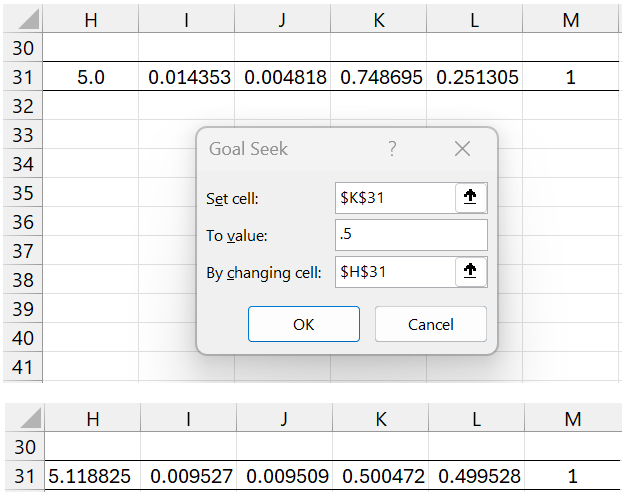
In fact, we can find the cutoff point between cluster 1 and cluster 2 by using Excel’s Goal Seek. To do this, we select Data > What-If Analysis|Goal Seek… Now fill in the dialog box that appears as shown on the upper part of Figure 7.

Figure 7 – Finding cutoff point using Goal Seek

After pressing the OK button, row 31 changes to the values shown on the bottom of the figure. The border between cluster 1 and 2 occurs at about 5.118825. Values below are in cluster 1 and those above are in cluster 2.

Examples Workbook

Click here to download the Excel workbook with the examples described on this webpage.

References

McGonagle, J. et al (2024) Gaussian mixture model
https://brilliant.org/wiki/gaussian-mixture-model/

Carrasco, O. C. and Whitfield, B. (2024) Gaussian mixture models explained
https://builtin.com/articles/gaussian-mixture-model

GeeksforGeeks (2023) Gaussian mixture model
https://www.geeksforgeeks.org/gaussian-mixture-model/

Apgar, V. (2023) 3 use-cases for Gaussian Mixture Models (GMM)
https://towardsdatascience.com/3-use-cases-for-gaussian-mixture-model-gmm-72951fcf8363