Supplementary Profiles
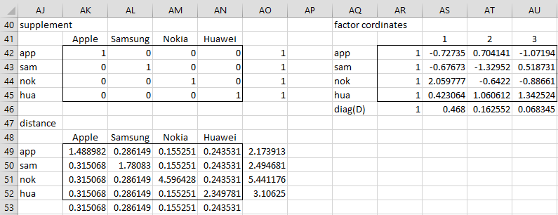
Instead of plotting row and column points on the same chart (as described in CA Plots), we can use supplementary profiles. E.g. we can add four supplemental points (app, sam, nok, hua) to the CA Rows plot for Example 1 of CA Basic Concepts, one for each of the smartphone brands as shown in range AJ41:AN45 of Figure 1.
Figure 1 – Supplementary rows
We next calculate the squared distances and factor coordinates of these supplementary profiles in a manner similar to how we calculated the squared distances and factor coordinates for the original profiles. E.g. the squared distance between app and the origin of 2.1667 (cell AD49) is calculated by the formula =SUM(AK49:AN49), where e.g. the formula in cell AK49 is =(AK42-AK$53)^2/AK$53 (and the values in range AK53:AN53 are the same as those in range P10:S10 of Figure 2 of CA Basic Concepts).
Similarly, the factor coordinates for the supplementary row points (range AR42:AY45) are calculated by the worksheet array formula =MMULT(AK42:AN45,AC20:AF23)/AR46:AU46 (where the values in range AR46:AU46 are the same as those in the diagonal of the matrix in range V32:Y35 of Figure 3 in CA Basic Concepts).
Supplementary Rows
We can use these values to create a report similar to that shown in Figure 6 of CA Basic Concepts for the original data. This report is shown in Figure 2.
Figure 2 – Detailed Report of the Supplementary Rows
The missing elements in the figure are for values that only occur in the original data.
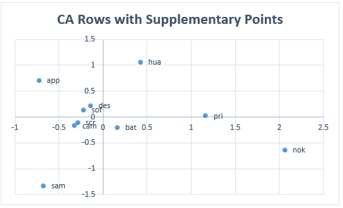
We can now create a plot of the original and supplementary row profiles as shown in Figure 3.
Figure 3 – CA Rows including supplementary points
Supplementary Columns
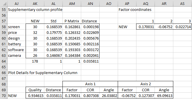
We can also create supplementary column profiles. E.g. if we have a new smartphone brand NEW with the characteristics shown in range AJ58:AK63 of Figure 4.
To calculate the coordinates for the NEW brand, first, we need to standardize the data by dividing each characteristic value by the total of the characteristic values (178 in this case). This yields the values in range AL58:AL63. Next, we copy the values from range T4:T9 of Figure 2 in CA Basic Concepts into range AM58:AM63 of Figure 4 and then calculate the squared distance of 0.0358 (cell AN64) by placing the formula =(AL58-AM58)^2/AM58 in cell AN58, highlighting the range AN58:AN63 and pressing Ctrl-D, and then placing the formula =SUM(AN58:AN63) in cell AN64.
Finally, we calculate the factor coordinates for NEW by placing the following array formula in range AQ58:AS58:
=MMULT(TRANSPOSE(AL58:AL63),AD12:AF17)/AS46:AU46
Figure 4 – CA Columns with supplementary brand
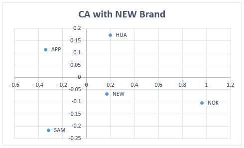
The revised CA plot is shown in Figure 5.
Figure 5 – CA Columns Plot including NEW brand
Examples Workbook
Click here to download the Excel workbook with the examples described on this webpage.
References
Hintze, J. L. (2007) Correspondence analysis. NCSS.
https://www.ncss.com/wp-content/themes/ncss/pdf/Procedures/NCSS/Correspondence_Analysis.pdf
Garson, G. D. (2012) Correspondence Analysis. Asheboro, NC: Statistical Associates Publishers.
Yelland, P. M. (2010) An introduction to correspondence analysis. The Mathematica Journal
https://www.mathematica-journal.com/2010/09/20/an-introduction-to-correspondence-analysis/


