Worksheet Functions
Real Statistics Functions: The Real Statistics Resource Pack contains the following array functions where R1 is an array containing an m × n contingency table, R2 is an mm × n array containing supplementary row profiles and R3 is an m × nn array containing supplementary column profiles. None of these arrays include row or column headings or totals. We also assume that k = min(m, n) – 1.
CARowFactors(R1): returns an m × k array in which the ith row contains the ith row factor vector for R1
CAColFactors(R1): returns an n × k array in which the ith row contains the ith column factor vector for R1
CARowFactors(R1, R2): returns an mm × n array in which the ith row contains the row factor vector for the ith supplementary row profile in R2 based on the data in R1.
CAColFactors(R1, R3): returns an m × nn array in which the ith row contains the factor vector for the ith supplementary column profile in R3 based on the data in R1.
CAEigen(R1): returns a k × 1 column array with the CA eigenvalues for R1
Data Analysis Tool
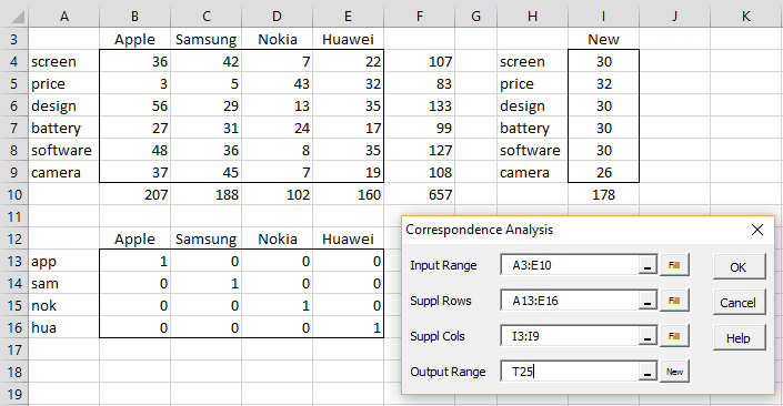
Real Statistics Data Analysis Tool: The Real Statistics Resource Pack provides the Correspondence Analysis data analysis tool which automates the steps described above. We show how to use this tool for Example 1 of CA Basic Concepts, where we have added a column profile as shown in range I3:I10 of Figure 1.
Press Ctrl-m (or an equivalent) and choose the Multivariate Analyses option from the original interface or the Multivar tab from the multipage interface. Now choose the Correspondence Analysis option to display the dialog box shown in Figure 1.
Figure 1 – Correspondence Analysis dialog box
We next fill in the Input Range with the contingency table in range A3:E10 (including row and column headings, but not including totals). The Suppl Rows and Suppl Cols fields are optional and can be left blank. For our example, we fill in the Suppl Rows field with the four supplementary row profiles in range A13:E16 (including row headings, but not column headings). We fill in the Suppl Cols field with the one supplementary column profile in range I3:I9 (including column headings, but not row headings or totals).
Analysis Output
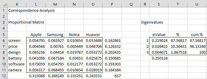
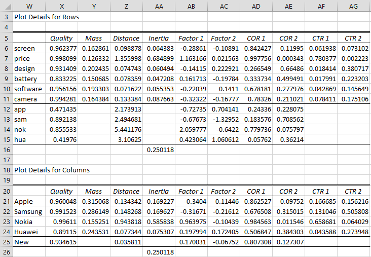
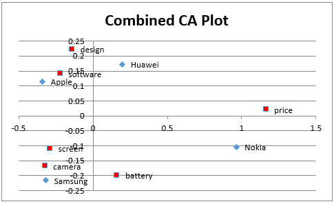
After pressing the OK button, the output in Figures 2 and 3 as well as the plots in Figures 4, 5, and 6 are displayed.
Figure 2 – Correspondence Analysis (part 1)
Figure 3 – Correspondence Analysis (part 2)
Formulas
Note that range S6:S8 contains the array formula =CAEigen(B4:E9), range AB6:AC11 contains the array formula =CARowFactors(B4:E9) and range AB12:AC15 contains =CARowFactors(B4:E9,B13:E16). Similarly, range AB21:AC24 contains the array formula =CAColFactors(B4:E9) and range AB25:AC25 contains =CAColFactors(B4:E9,I4:I9).
Note too that cell Z12 contains the array formula
=SUMPRODUCT((B13:E13/SUM(B13:E13)-L$12:O$12)^2/L$12:O$12)
and cell Z25 contains
=SUMPRODUCT((I4:I9/SUM(I4:I9)-P6:P11)^2/P6:P11)
Plots
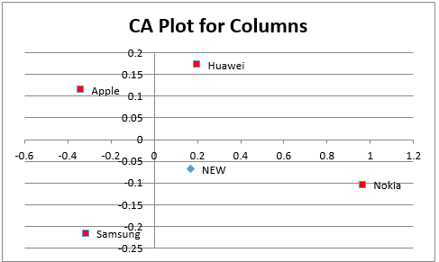
Using these results we create the CA plots for rows and columns shown in Figures 4 and 5.
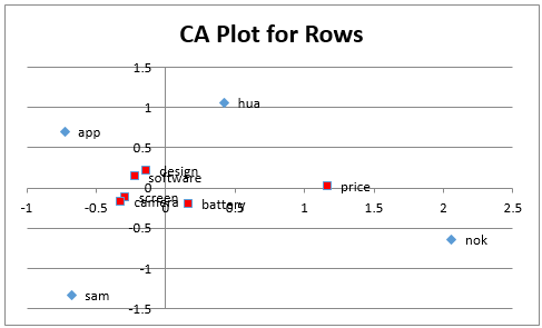
Figure 4 – Correspondence Analysis (part 3)
Figure 5 – Correspondence Analysis (part 4)
as well as the combined plot shown in Figure 6.
Figure 6 – Correspondence Analysis (part 5)
Examples Workbook
Click here to download the Excel workbook with the examples described on this webpage.
References
Hintze, J. L. (2007) Correspondence analysis. NCSS.
https://www.ncss.com/wp-content/themes/ncss/pdf/Procedures/NCSS/Correspondence_Analysis.pdf
Garson, G. D. (2012) Correspondence Analysis. Asheboro, NC: Statistical Associates Publishers
Yelland, P. M. (2010) An introduction to correspondence analysis. The Mathematica Journal
https://www.mathematica-journal.com/2010/09/20/an-introduction-to-correspondence-analysis/
