Basic Concepts
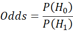
Hypothesis testing consists of determining whether the null hypothesis H0 is more likely or less likely than an alternative hypothesis H1 and by how much. Before we collect data, we compare P(H0) with P(H1) based on our prior beliefs as described by the prior probability functions for each hypothesis. We define the prior odds by
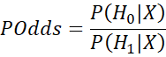
Once we have collected some data X, we can compare the posterior probabilities. Based on these, we can define the posterior odds by
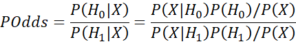
Using Bayes Theorem, it follows that
Bayes Factor
Thus, the posterior odds are equal to the Bayes Factor (BF) times the prior odds, where the Bayes Factor is the ratio between the likelihood functions, i.e. BF compares the evidence between the two hypotheses.
When the hypotheses involve a parameter (or a number of parameters), then BF is a ratio of the marginal probabilities, and so BF is defined in the discrete and continuous cases by
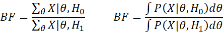
Thus, BF takes into consideration all possible values of the parameters (based on each hypothesis).
Figure 1 shows a way of evaluating the Bayesian Factor as a substitute for evaluating p-values in frequentist statistics. There are various alternative versions of this table (especially by replacing 3.2 and 32 by 3 and 30).
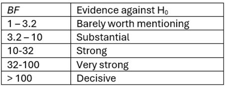
Figure 1 – Interpreting the Bayes Factor
Example
Example 1: Let’s revisit Example 1 of about HIV testing, and in particular let’s consider the patients that tested positive for the virus. We will test the hypothesis that the patient doesn’t have HIV (hypothesis H0) vs. the patient does have HIV (hypothesis H1).
The prior probabilities are P(H1) = .00148 and so P(H0) = 1 – .00148 = .99852. Thus, the prior odds are
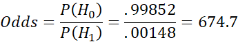
This means that prior to obtaining any test results it is 674.7 times more likely that a patient doesn’t have HIV (hypothesis H0) than the patient has HIV (hypothesis H1).
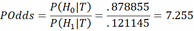
Now let T represent the event that the test is positive. In Example 1, we found that P(H1|T) = .121145 and so P(H0|T) = 1 – .121145 = .878855 (see Bayesian Example). Thus, the posterior odds are now
Since POdds = BF ⋅ Odds, if follows that
![]()
Note too that since the false positive rate for a HIV test is 7% and the false negative rate is 1%, we see that
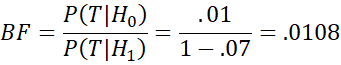
which is the same result.
Notation
Henceforth, we will use the notation BF01 for the version of the Bayes Factor described above as the inverse BF10 = 1/BF01.
References
Reich, B. J., Ghosh, S. K. (2019) Bayesian statistics methods. CRC Press
Wikipedia (2024) Bayesian factor
https://en.wikipedia.org/wiki/Bayes_factor
Lee, P. M. (2012) Bayesian statistics an introduction. 4th Ed. Wiley
https://www.wiley.com/en-us/Bayesian+Statistics%3A+An+Introduction%2C+4th+Edition-p-9781118332573