Bayesian Independence Testing

Objective

We describe the Bayesian approach to determining whether the two variables defined by a contingency table are independent. This is the Bayesian equivalence to the chi-square test of independence or Fisher’s exact test. See also Bayesian Hypothesis Testing.

Terminology

We assume that we have an m × n contingency table X = [x_ij] and want to test the following hypotheses:

H₀: Row/column independence

H₁: Row/column dependence

We now define

We also assume priors A = [a_ij], and define similar quantities for the A matrix to those described above for the X matrix. In addition, we define the following:

Finally, for any m × n matrix Y = [y_ij], we define

and for any vector Y = [y_i], we define

Example

We explain this terminology further using the contingency table in Figure 1.

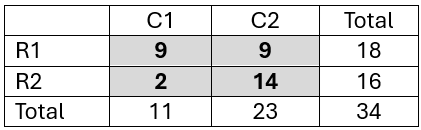
Figure 1 – Contingency Table

Based on the above terminology, we see that

x₂₁ = 2, x_.1 = 11, x_T = 34, X_col = (11, 23), m = n = 2

If a_ij = 1 for all i,j, then a_T = 4, A_row = A_col = (2,2)

C_row = (2-1, 2-1) = (1, 1), c = 4-1 = 3

D(X_row) = Γ(18) ⋅ Γ(16) / Γ(34) = 17!15!/33! = 5.34652E-11

We now show how to test the independence hypotheses described above using several different approaches.

Poisson sampling

In this sampling approach, we assume that none of the cell counts are fixed. We assume that the cell counts follow a Poisson distribution where the mean/rate parameters λ_ij have a gamma distribution with shape parameters a_ij and scale parameter b.

x_ij ∼ Poisson(λ_ij)

λ_ij ∼ Gamma (a_ij, b)

We assume that all the a_ij are the same with value a (default 1), and that the default for b is

b = mna/x_T

The Bayes Factor for this sampling approach is

For a 2 × 2 contingency table with a = 1, it follows that

Example

Example 1: Calculate BF₀₁ for the contingency table in range B2:D3 of Figure 2 based on the prior parameter a = 1.

We show the table of priors including totals in range B7:E9. Range F7:F8 contains C_row, B10:D10 contains C_col, and cell F10 contains c. The right side of the figure calculates BF₀₁ as a product of the 5 terms in the above formula. To simplify the calculations we use the DFunc worksheet function defined below.

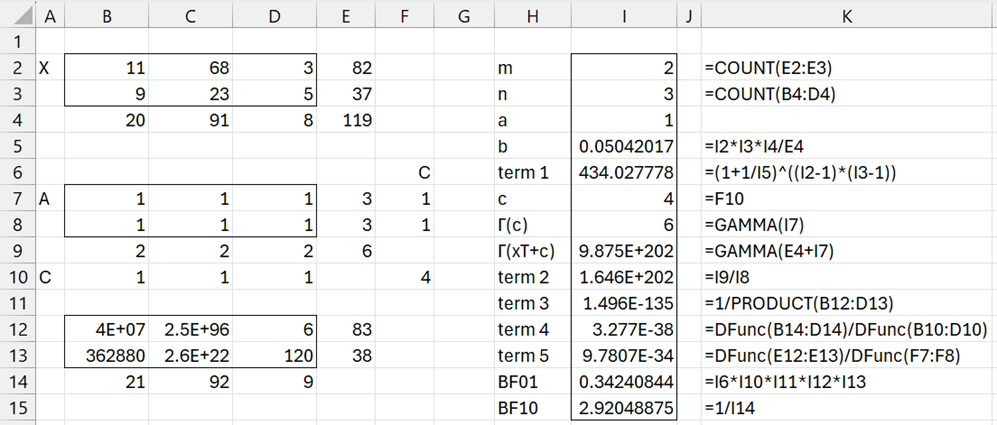Figure 2 – Poisson sampling example

Joint multinomial sampling

In the joint multinomial sampling approach we assume that only the grand total x_T is fixed and

(x₁₁, …, x_mn) ∼ Multinomial(x_T, π)

where π takes a Dirichlet distribution:

π ∼ Dirichlet(a₁₁, …, a_mn)

In this case

For a 2 × 2 contingency table with a = 1, it follows that

Independent multinomial sampling

This time, we assume that either the row or column totals are known. If the row totals are known then

If the column totals are known then

For a 2 × 2 table with a = 1

Hypergeometric sampling

This time we assume that all marginal totals are fixed.

For a 2 × 2 table with a = 1

where we have chosen x_1. to be the smallest of the marginal totals.

Worksheet Functions

Click here for a description of worksheet functions and data analysis tools that can be used to perform Bayesian independence testing in Excel.

Examples Workbook

Click here to download the Excel workbook with the examples described on this webpage.

References

Jamil, T., Ly, A., Morey, R. D., Love, J., Marsman, M., Wagenmakers, E-J. (2016) Default “Gunel and Dickey” Bayes factors for contingency tables
https://www.alexander-ly.com/wp-content/uploads/2014/09/JamilEtAlGunelDickeyinpress.pdf

Albert, J. (2009) Bayesian computation with R, 2^nd ed. Springer