Introduction
In Two Factor ANOVA without Replication, we consider the analysis where there is only one sample item for each combination of factor A and B levels. On this webpage, we extend this analysis to the case where there are multiple samples for each such combination. Thus, in addition to the main effects corresponding to A and B, we now study the interactions between A and B, which is the main reason for performing this type of analysis.
We will restrict ourselves to the case where all the samples are equal in size (balanced model). In Unbalanced Factorial ANOVA we show how to perform the analysis where the samples are not equal (unbalanced model) via regression.
You should not confuse ANOVA with replication with ANOVA with repeated measures as described in ANOVA with Repeated Measures.
Example introduced
As usual, we start with an example. We then provide some background information and then complete the analysis for the example.
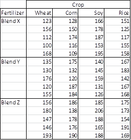
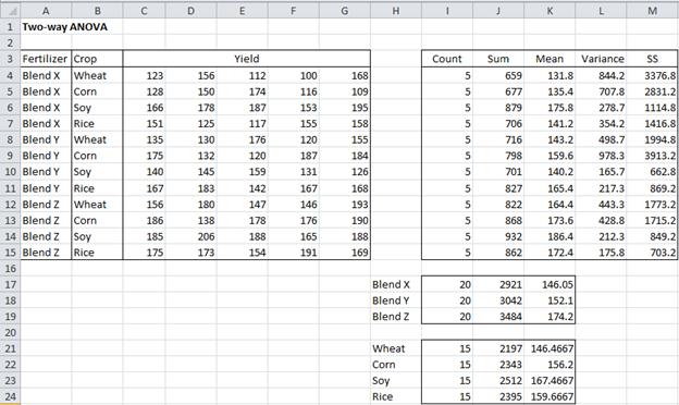
Example 1: Repeat the analysis from Example 1 of Two Factor ANOVA without Replication, but this time with the data shown in Figure 1 where each combination of blend and crop has a sample of size 5.
Figure 1 – Data for Example 1
Structural Model
Definition 1: We extend the structural model of Definition 1 of Two Factor ANOVA without Replication as follows.
In Definition 1 of Two Factor ANOVA without Replication the r × c table contains the entries {xij: 1 ≤ i ≤ r, 1 ≤ j ≤ c}. We extend these tables to contain entries {Xij: 1 ≤ i ≤ r, 1 ≤ j ≤ c}, where Xij is a sample for level i of factor A and level j of factor B. Here Xij = {xijk: 1 ≤ k ≤ nij}. For now, we assume the nij are all equal of size m.
We use terms such as x̄i (or x̄i.) as an abbreviation for the mean of {xijk: 1 ≤ j ≤ c, 1 ≤ k ≤ m}. We also use terms such as x̄j (or x̄.j) as an abbreviation for the mean of {xijk: 1 ≤ i ≤ r, 1 ≤ k ≤ m}.
As in Definition 1 of Two Factor ANOVA without Replication, we define the effects αi and βj where
Similarly, we define ai and bj where
We use δij for the effect of level i of factor A with level j of factor B, i.e. the interaction of level i of factor A and level j of factor B. Thus, δij = μij – μi – μj + μ. Similarly, we have
It is easy to show that
![]()
Finally, we can represent each element in the sample as
where εijk denotes the error (or unexplained) amount. As before we have the sample version
where eijk is the counterpart to εijk in the sample. Note that
Null Hypotheses
As in Definition 1 of Two Factor ANOVA without Replication, the null hypotheses for the main effects are:
H0: μ1. = μ2. = … = μr. (Factor A)
H0: μ.2 = μ.2 = … = μ.c (Factor B)
These are equivalent to:
H0: αi = 0 for all i (Factor A)
H0: βj = 0 for all j (Factor B)
In addition, there is a null hypothesis for the effects due to the interaction between factors A and B.
H0: δij = 0 for all i, j
More about the structural model
Definition 2: Using the terminology of Definition 1, define
We can also define the following entities:
Since the within groups terms are used as the error terms in our model, we also use the following symbols:
![]()
Properties
Property 1:
Proof: Clearly
If we square both sides of the equation, sum over i, j, and k, and then simplify (with various terms equal to zero as in the proof of Property 2 of Basic Concepts for ANOVA), we get the first result. For the second,
Property 2: Note that the between-group terms are as for the one-way ANOVA, namely
The proof is similar to the proof of Property 1. It also follows that
![]()
Property 3: If a sample is made as described in Definitions 1 and 2, with the xijk independently and normally distributed and with all (or
) equal, then
Proof: The proof is similar to that of Property 1 of Basic Concepts for ANOVA.
Property 4: Suppose a sample is made as described in Definitions 1 and 2, with the xijk independently and normally distributed.
If all μi are equal and all are equal then
If all μj are equal and all are equal then
Also, under certain circumstances,
Proof: The result follows from Property 3 and Property 1 of F Distribution.
Property 5:
Statistical Tests
We use the following tests:
Assumptions
The assumptions for Two Factor ANOVA are similar to those for One Factor ANOVA, namely
- All samples are drawn from normally distributed populations
- The samples are drawn from populations that have a common variance
- All samples are drawn independently from each other
- Within each sample, the observations are sampled randomly and independently of each other
By sample, here we mean each combination of levels from the two factors. We also want to make sure there are no outliers that can distort the results of the test. See ANOVA Assumptions for how we check these assumptions using the Real Statistics Resource Pack.
Example continued
We now return to Example 1 and show how to conduct the required analysis using Excel’s Anova: Two-factor With Replication data analysis tool.
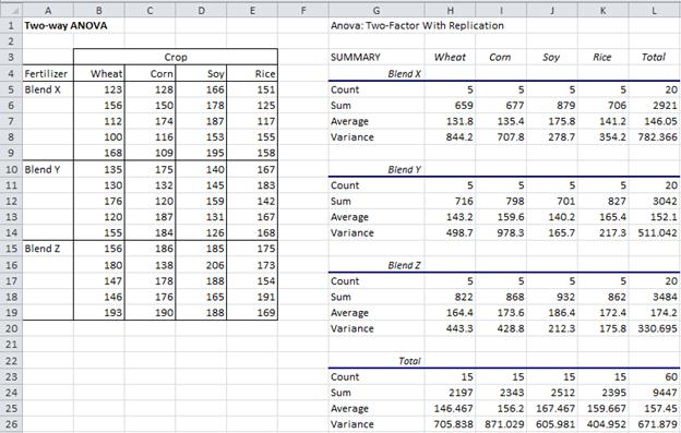
Example 1 (continued): The summary output from the data analysis tool is given on the right side of Figure 2, with the sample data repeated on the left side of the figure.
Figure 2 – Summary output of ANOVA data analysis for Example 1
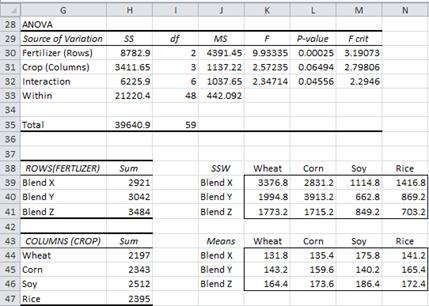
The top part of Figure 3 contains the rest of the output from the data analysis tool. We’ll explain the bottom part momentarily.
Figure 3 – ANOVA analysis for Example 1
We now draw some conclusions from the ANOVA table in Figure 3. Since the p-value (crops) = .0649 > .05 = α, we can’t reject the Factor B null hypothesis, and so conclude (with 95% confidence) that there are no significant differences between the effectiveness of the fertilizer for the different crops.
Since the p-value (blends) = .00025 < .05 = α, we reject the Factor A null hypothesis and conclude that the blends are statistically different.
Interaction Plots
We also see that the p-value (interactions) = .0456 < .05 = α, and so conclude there are significant differences in the interaction between crop and blend. We can look more carefully at the interactions by plotting the mean interactions between the levels of the two factors (see Figure 4). Lines that are roughly parallel are indications of the lack of interaction, while lines that are not roughly parallel indicate interaction.
From the first chart we can see that Blend Y has quite a different pattern from the other brands, especially since the line for Blend Y is trending down towards Soy and up towards Rice, exactly the opposite of Blend X and Z). We also see that Blend X is trending up towards Soy much more abruptly than Blend Z.
Figure 4 – Interaction plots for Example 1
Worksheet Functions
Although the analysis in Figures 2 and 3 was produced automatically by Excel’s data analysis tool, the same result can be produced using Excel formulas, just as we were able to do for Example 1 of Two Factor ANOVA without Replication. In fact, all the entries in the ANOVA table in Figure 3 can be calculated using the tables constructed in the bottom part of Figure 3 in exactly the same way as was done in Example 1 of Two Factor ANOVA without Replication.
In fact, the only thing new is the calculation of the error term SSW. To calculate it we must first construct the table of the square deviations for all the interactions from their mean. This table appears in cells J38:N41 of Figure 3. E.g. the entry for SSWheat,BrandX (in cell K39) is =DEVSQ(B5:B9). SSW is then calculated as the sum of all the terms in the table, namely =SUM(K39:N41).
Alternatively, we can use Property 2 to calculate SSBet and then use the fact that SSW = SST – SSBet. To calculate SSBet we first construct the table of the means of the various interactions of factors A and B (range J43:N46 of Figure 3), as described below. SSBet is now calculated using the formula =DEVSQ(K44:N46)*H5. For Example 1, SSBet = 18420.5, and so SSW = SST – SSBet = 39640.9 – 18420.5 = 21220.4.
Example using row formatting
Example 2: Repeat the analysis for the data in Example 1 by using the presentation of the data given in the table on the left of Figure 5.
Figure 5 – Alternative presentation of data in Example 1
Excel’s ANOVA data analysis tools don’t support data in this format, and so we must proceed to create the ANOVA table (i.e. the output found in Figure 3) using the formulas. This is straightforward, although tedious, with the result presented in Figure 6. As usual, the hardest part is the calculations for the SS terms, which are shown on the right side of the worksheet in Figure 6.
Figure 6 – ANOVA output for Example 2
When the assumptions are not met
In general, when the assumptions are violated, transformations and non-parametric (rank) tests are not very useful for two-way ANOVA. We can instead abandon the omnibus test and apply the various planned and unplanned tests described in Planned Comparisons for ANOVA and Unplanned Comparisons for ANOVA by treating the two-way ANOVA as a one-way ANOVA.
In particular, when the variances are not equal we can apply Welch’s correction for contrasts. We can also use the Scheirer-Ray-Hare test or Aligned Rank Transform (ART) ANOVA
Examples Workbook
Click here to download the Excel workbook with the examples described on this webpage.
References
Howell, D. C. (2010) Statistical methods for psychology (7th ed.). Wadsworth, Cengage Learning.
https://labs.la.utexas.edu/gilden/files/2016/05/Statistics-Text.pdf
Tutorialpoint (2024) How to conduct ANOVA two-factor with replications in Excel
https://www.tutorialspoint.com/how-to-conduct-anova-two-factor-with-replication-in-excel
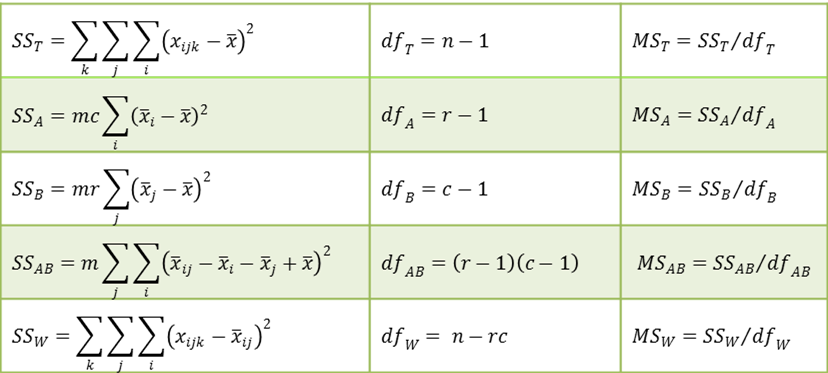



I believe the formula for SS.AB in Definition 2 is incorrect if the values in Figure 3 are correct for the example. I believe there should not be an ‘m’ in front of the summations so it should be SS.AB = sum sum (xbar.ij – xbar.i – xbar.j – xbar)^2
Sonia,
I just checked the calculations in Figure 3 and found that the formula in Def 2 for SS.AB is correct. The m is needed.
Please check your calculations. If you still don’t get the results in Figure 3, I will share the calculations that I made.
Charles
Hi Charles,
The post says “By sample, here we mean each combination of levels from the two factors”.
But when it comes to Two Factor ANOVA without Replication, how can “sample” be defined and how can we check the assumptions with only one subject in each combination of levels?
Hi,
You just need to check the assumptions for each factor since there is no interaction.
The assumptions for two factor ANOVA without replication is briefly described at
https://real-statistics.com/two-way-anova/two-factor-anova-without-replication/
Charles
Very clear answer.
The piont is at “there is no interaction”.
Great thanks!
Dear Professor,
Is this not 2 one- way ANOVAs with the first ANOVA done with the data table being read upright and the second with the data table read crosswise (sideways)?
Curious.
Ray
oops, i was commenting on the two way ANOVA without replication . sorry , wrong page.
Ray
Hi Ray,
Do you still have a question or comment?
Charles
Hello, I am a little confused about paragraph before Figure 4. because it aapears …especially since the line for Blend Y is trending up towards Soy and down towards Rice, exactly the opposite of Blend X and Z)…
However, it can be seen that the trend is the opposite: Blend Y is trending down towards Soy and up towards Rice. Am I right or is my interpretation wrong?
Hello Juan,
The statement should be “…line for Blend Y is trending down towards Soy and up towards Rice, exactly the opposite of Blend X and Z)…”
I have changed the webpage to fix this error. Thanks for your comment, which made me aware of the incorrect and confusing statement.
Charles
how you draw the charts?
Hello Suzi,
I used Excel’s charting capabilities as described at
Excel Charts
Charles
Dear Charles,
I designed an experiment in order to study differences in ovarian follicular population related to age of women. So, we have 3 ages (young, adult and old) as independent variable and 3 follicular sizes (small, medium and big) as dependent variable. In addition, the model must include the effect of body condition ranked of 1 (very thin) to 5 (obese) and days post-partum, as covariate.
I’m not sure which statistics of the Real Statistics package I should use. Can you help me?
Thanks.
Hello Rafael,
It depends on what hypothesis or hypotheses you want to test.
If I understand correctly, you have two factors: Age (3 levels) and Body Condition (5 levels). Your dependent variable seems to take 3 ordered values (0,1,2). You might be able to use ordinal regression, but it all depends on what you are trying test.
Charles
Wonderful work! Very instructive!
Only one question about your last observation : do the methods for multiple comparisons need to meet the normality assumption?
If it is necessary, I think we cannot use these methods when the normality assumption is violated.
Hello Xi,
Glad you are getting value from the website.
Yes. It is assumed that multiple comparisons were done after a significant ANOVA result. ANOVA requires normality.
These tests are pretty robust to violations of normality, and so it depends on how far from normality you are.
Charles
Thanks!
Good morning Charles,
Is this the case when I have a Randomized Complete Block Design with 5 replicates?
(i.e.: the five yield values for each fertilizer/crop combination come from replicates in the same experimental design?)
Thanks a lot for your support with the awesome website!
Guido
Hello Guido,
If I understand your question correctly, then I believe the answer is “yes”. This type of approach is explained at
https://www.real-statistics.com/design-of-experiments/completely-randomized-design/randomized-complete-block-design/
Charles
Thanks a lot!
so there are 5 replicates?
Yes
It might be useful to make clear at the top of this post that “with replication” and “repeated measures” are not the same thing. This is especially important because the 2-factor ANOVA with replication function in Excel appears to perform that function well for multiple independent observations per cell, but not when, for example, a group of subjects is tested under multiple conditions were each person serves as his or her own control. Excel does not seem to be able to correctly perform a 2-factor ANOVA with repeated measures.
Excel seems to perform 1-factor ANOVA with repeated measures satisfactorily, although as you point out, the procedure is misnamed.
Hi Marvin,
Thanks for your comment. I have now revised the webpage as you have suggested.
Charles
Hi, I am using a two way anova to look at changes in blood pressure over time. I have the same issue with the p value showing #NUM!.
Hannah,
If you email me an Excel file with your data and test results I will try to figure out why you are getting this error value.
Charles
Hi I’m using two way anova for difference in infiltration rates across three plots before and after human trampling. I have three infiltration values before trampling and three infiltration values after trampling but when i calculate the anova #NUM ! appears in the P-values and F crit boxes, could you please help? Thank you.
The data i’m using is: Plot 1: 8.5 and 0.7, Plot 2: 2.6 and 0.4 and Plot 3; 2.5 and 2.1
Charlotte,
If you email me an Excel file with your data and results, I will try to figure out what is going wrong.
Charles
Dear Sir,
How to calculate precision based on ANOVA output of excel?
Sorry, but I don’t understand the context of your question. What sort of precision are you referring to?
Charles
Dear Sir,
Sorry, I have asked question in wrong segment. I was referring to Two factor nested ANOVA model. Considering experiment is done twice a day in two replicates and that for 20 days. That data is analysed by two factor nested ANOVA. The output that comes as summary table. From this how to calculate SD and CV with respect to Repeatibility and Precision. Hope I am able to explain you…
Hello Shailesh,
Does the following webpage address your issue?
https://www.real-statistics.com/two-way-anova/gage-rr/
Charles
Thank you Charles….
In last example what was number of row per sample
Anand,
As explained in the paragraph right after Figure 5, I didn’t use the Excel ANOVA tool (and so the number of rows per sample is not relevant). Instead, I used certain formulas.
Charles
Thanks for nice information…….I would like to tell you that I have two years of above like data, then how i make combined analysis for two years i.e. Two factor lab data of two years. Please suggest me.
What hypothesis do you want to test?
Charles