On this webpage, we describe Real Statistics support for Two-Factor ART ANOVA.
Worksheet Function
Real Statistics Function: The Real Statistics Resource Pack supports the following array function:
Std2Art(R1, head): takes the data in R1 in standard two-factor ANOVA format (i.e. a three-column array whose first two columns consist of the row and column factor labels, and whose third column consists of the corresponding values of the dependent variable) and returns an array with five columns, the first two columns are identical to the first two columns of R1 and the other columns are the ART ranks for rows, columns and interactions; if head = TRUE (default FALSE) then both R1 and the output contain column headings.
You can obtain the results shown in range J25:L42 of Figure 1 of Two-Factor ART ANOVA by using the array formula =Std2Art(A25:C42).
Data Analysis Tool
Real Statistics Data Analysis Tool: ART ANOVA can be performed by using the ART ANOVA option of the Two-Factor ANOVA data analysis tool.
For Example 1 of Two-Factor ART ANOVA, press Ctrl-m and choose the Two-Factor ANOVA option from the Anova tab. This brings up the dialog box shown in Figure 1.
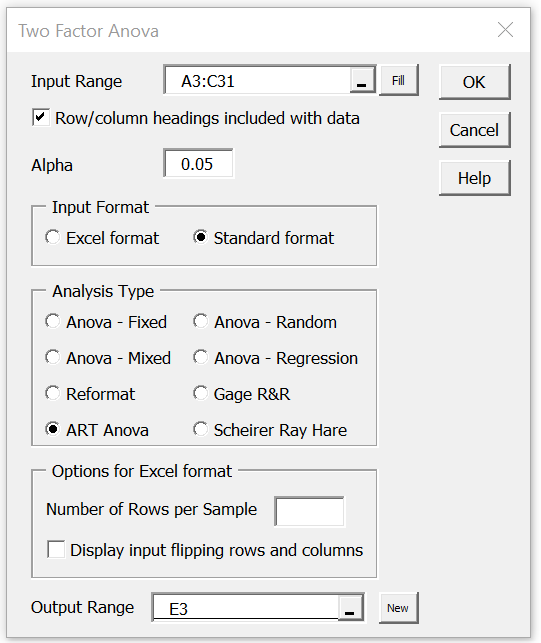
Figure 1 – ART option of Two-Factor ANOVA dialog box
Now, fill in the dialog box as shown in the figure and click on the OK button. The output is displayed in Figure 2.
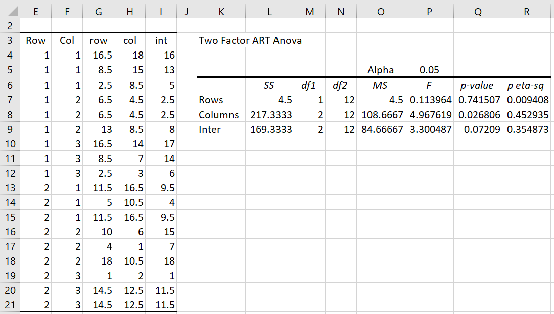
Figure 2 – ART ANOVA output
Examples Workbook
Click here to download the Excel workbook with the examples described on this webpage.
References
Wobbrock, J. O., Findlater, L., Gergle, D., Higgins, J. J. (2011) The Aligned Rank Transform for Nonparametric Factorial Analyses Using Only ANOVA Procedures. Conference: Proceedings of the International Conference on Human Factors in Computing Systems, CHI 2011, Vancouver, BC, Canada
https://faculty.washington.edu/wobbrock/pubs/chi-11.06.pdf
Leys, C. and Schumann, S. (2010) A nonparametric method to analyze interactions: The adjusted rank transform test
http://cescup.ulb.be/wp-content/uploads/2015/04/Leys_and_Schumann_nonparametric_interactions.pdf
Has something changed recently in your Excel formulas for the sums of squares? About one month ago, I performed an ART ANOVA and received results that were consistent with SPSS when the aligned ranks were passed through the general linear model procedure.
Today, when I ran your ART ANOVA on the same data, the sums of squares are incorrect and the interaction sum of squares is even negative!
For reference, your previous interaction sum of squares cell formula was =INDEX(SSAnova2(MERGE(E2:F275,I2:I275)),3). Now, it’s =@SSIntStd(MERGE(E2:F275,I2:I275))
Hi Craig,
Thanks for bringing this issue to my attention. Unfortunately, I don’t fully understand where these formulas are coming from. I downloaded the workbook from this webpage and found that the closest formula to the one you referenced appears in cell L9. The formula there is
=@SSIntStd(MERGE(E4:F21,I4:I21)). I then entered the formula =INDEX(SSAnova2(MERGE(E4:F21,I4:I21)),3). In both cases I got the same result, namely 169.333. Is this what you got? Is this consistent with the results from SPSS?
BTW, I have not made any changes to these formulas in the past month. The workbook was create in February of this year.
Charles
Charles,
I realize that although I performed the analysis a month ago, it was on a different computer, so it was using your older formula. I am referencing cell L9 in your example. Maybe it’s tied to the size of the dataset? When I run your current formula on a dataset of more than 200 observations, I get a negative sum of squares, but when I copy and paste your old formula into the “L9” cell, I get the correct value. I do get the correct value using both formulas for your example dataset. For some reason, the row and column sums of squares are unaffected.
Craig
I have to amend my prior comment. Both the row and column sums of squares are also incorrect. To correctly replicate SPSS, I had to copy your old “L” and “P” column formulas into my current spreadsheet.