Engle-Granger Test

Cointegration

When establishing the relationship between two time series, we may find that neither is stationary, but at any point in time they have values that are close to each other, and, in fact, even when one drifts away from the other, it tends to come back.

This is similar to a man who is walking his dog on a leash. Even if both are following a random walk, the leash guarantees that they never get too far apart. This is also true of many economic time series.

Cointegration Testing

Formally, we define that two times series are cointegrated when

1. neither time series is stationary
2. their first differences are stationary
3. the time series consisting of the residuals from the linear regression of one of the time series on the other is stationary

As we will see, we can use the ADF test for steps 1 and 2 and a modified version of the ADF test for step 3. The modification is that a different table of critical values needs to be employed for step 3, as explained below. This three-step approach is called the Engle-Granger Test.

Examples

Example 1: Determine whether the daily price per barrel of Brent crude oil is cointegrated with the price per barrel of WTI (Western Texas Intermediate) crude oil over the period 2009-2010.

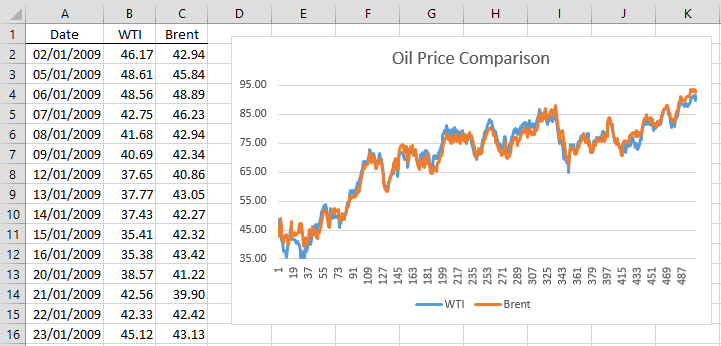
Figure 1 shows the daily prices of these two commodities (only the first 15 of 504 daily price comparisons are shown in the figure) along with a time series plot.

Figure 1 – Time series plot 

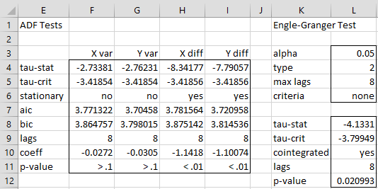
The plot shows the potential that the two time series are cointegrated. To test this, first, we use the ADF test to determine whether each time series is not stationary, but their first differences are stationary. The results of the four tests are shown on the left side of Figure 2.

Figure 2 – ADF Tests

From columns F and G, we see that the two series are not stationary, but from columns H and I, we see that their first differences are stationary. Here, range E4:F11 contains the Real Statistics worksheet array formula =ADFTEST(B2:B505,TRUE,L5,L6,L4,L3). We choose the maximum number of lags for the test to be 8 (cell L5), i.e. the cube root of the size of the time series, which in this case is 504, raised to the next highest integer. As we can see from Figure 1, both time series have a drift and a trend, and so we use type = 2 (cell L4).

Similarly, range G4:G11 contains the worksheet array formula =ADFTEST(C2:C505,,L5,L6,L4,L3). For the differenced time series, we use the array formula =ADFTEST(ADIFF(B2:B505),,L5,L6,L4,L3) in range H4:H11 and =ADFTEST(ADIFF(C2:C505),,L5,L6,L4,L3) in range I4:I11.

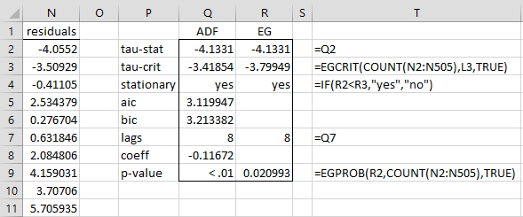
Now that we have shown the validity of requirements 1 and 2, we now perform the linear regression of the Y time series (Brent) on the X time series (WTI) to obtain the residuals, as shown in range N2:N505 of Figure 3 (only the first 10 residuals are displayed).

Figure 3 – Engle-Granger Test (step 3)

Range N2:N505 contains the worksheet array formula =C2:C505-TREND(C2:C505,B2:B505). We now perform the ADF test on this time series using the formula =ADFTEST(N2:N505,TRUE,8,,2) as shown in range Q2:Q9.

The two original times series are now considered to be cointegrated provided the residuals time series is stationary, which seems to be the case from cell Q4. As described previously, though, we can’t simply use the critical values for the ADF test (see Augmented Dickey-Fuller Table). Instead, we need to use the critical values by MacKinnon shown in Engle-Granger Table. Note that unlike the MacKinnon table used for the ADF test, this table only contains two types: with a trend and without a trend.

We can also use the following Real Statistics functions to calculate the critical values as well as approximate p-values based on these critical values.

Worksheet Functions

Real Statistics Functions: The Real Statistics Resource Pack supports the following two functions:

EGCRIT(n, alpha, tr) = critical value of the Engle-Granger test for two time series of length n for the significance level alpha (between .01 and .10, default .05) based on either a trend (when tr = TRUE) or no trend (when tr = FALSE, default)

EGPROB(t, n, tr) = estimated p-value of the Engle-Granger test for two time series of length n when the test statistic is t, where tr is as for EGCRIT.

Using these functions we obtain the result shown in column R of Figure 3. We see that the Engle-Granger Test concludes that the residuals are stationary, and so the two types of oil time series are cointegrated.

We can also use the following Real Statistics array function to obtain this result directly:

EGTEST(Rx, Ry, lab, lag, criteria, trend, alpha): outputs a column array with the values tau-stat, tau-critical, cointegrated (yes/no), lags, p-value

Here, Rx and Ry are column arrays containing the two time series, while lab, lag, criteria and alpha are as for the ADFTEST function (for the Augmented Dickey-Fuller Test) and tr = TRUE if there is a trend (default FALSE).

The results of the test for Example 1 can be found in range L8:L12 of Figure 2 by using the array formula =EGTEST(B2:B505,C2:C505,TRUE,L5,L6,L4,L3).

Data Analysis Tool

Real Statistics Data Analysis Tool: The Real Statistics Resource Pack provides the Cointegration data analysis tool which performs the Engle-Granger Test.

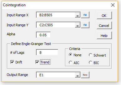
To perform the Engle-Granger Test for Example 1, press Ctrl-m and select the Cointegration data analysis tool from the Time S tab (or the Time Series data analysis tool if you are using the original user interface). Fill in the dialog box that appears as shown in Figure 4.

Figure 4 – Cointegration dialog box

After clicking on the OK button, the output shown in Figure 2 is displayed.

References

Mann, J. (2015) Video 7 – Cointegration. Gretl Instructional Series
https://www.youtube.com/watch?v=bJgx3JLb7fI
Gonzalo, J. (2014) Cointegration and error correction.
No longer available online
Buck, A. J. (1999) Cointegration and error correction
Engle, Granger (1987) Co-integration and error correction: representation, estimation, and testing
https://users.ssc.wisc.edu/~bhansen/718/EngleGranger1987.pdf
Is it possible to see the full p-value, when I conduct a engle-granger test it always comes out with >.1 or <.01
Tom,
This value is based on a table lookup, and so I don’t have any better information. If you have a source with better precision, I would gladly include this in the software.
Charles
Thank you so much for sharing this, the article is very well explained and easy to understand.
I have a question about ADF Test: You use a lag number of 8, which is the cube root of the size of the time series rounded upwards. Is there a reason for using this number? Is it some kind of standard or is it just an arbitrary choice?
Thanks again, regards!
Hello Jorge,
It is not arbitrary. It is a heuristic, but I don’t recall who came up with it.