Data Analysis Tool
Real Statistics Data Analysis Tool: The Real Statistics Resource Pack provides the Time Series Testing data analysis tool which consolidates many of the capabilities described in this part of the website.
Example 1
To use this tool for the data in Example 1 of Stationary Process (repeated in Figure 1), press Ctr-m and choose the Testing option from the Time S tab (or from the Time Series option if using the original user interface) and click on the OK button. Now, fill in the dialog box that appears as shown in Figure 1.
In Figure 1 we have inserted the time series values in the Input Range field, without column heading or date information. You can optionally request the ACF, ACVF and/or PACF values by placing a positive integer value in the corresponding field. In Figure 1 we have requested the ACF(k) values for lags k = 1, 2, 3, 4, 5. We could have requested any combination of ACF, ACVF or PACF values, or none at all.
Similarly, we can request any combination of the white noise tests (Bartlett’s, Box-Pierce, Ljung-Box) or none at all by inserting a positive integer in the corresponding field. In Figure 1 we have requested only the Ljung-Box test on ACF for lags up to 5.
Finally, we can optionally request the ADF test by inserting a non-negative integer value (including 0) in the # of Lags field or by leaving this field empty and selecting the Schwert option. We can also request to use the Drift or Trend options of the test. In Figure 1, we have requested the test with drift based on the number of lags specified by the Schwert criterion.
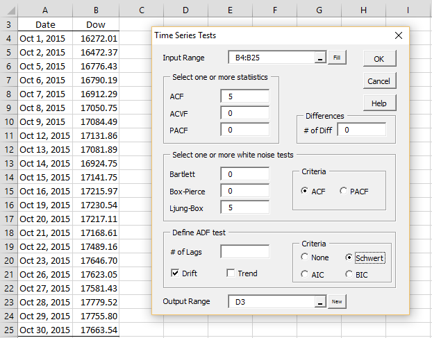
Figure 1 – Time Series Testing data analysis dialog box
The Schwert criterion calculates the lag based on the Excel formula
=ROUND(12 * (n / 100) ^ (1 / 4), 0)
which in this case is ROUND(12*(22/100)^(1/4),0) = 8. The AIC criteria is then used with lags = 8.
Output
The output for this analysis is shown in Figure 2 (only the first 15 of the 22 data elements are shown in columns D and E).
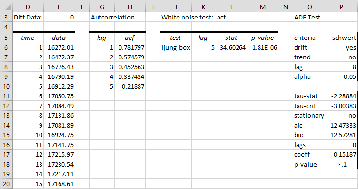
Figure 2 – Time Series data analysis
The first 5 ACF values are shown in column H. The Ljung-Box test gives a significant result (cell M6), which means that at least one of the first 5 autocorrelations is significantly different from zero. The Augmented Dickey-Fuller test shows that the time series is not stationary (cell P13).
Differencing
Example 2: Repeat Example 1 on the first differences of the data in Example 1.
We fill in the dialog box shown in Figure 1 with two changes, namely we change the # of Diff field from the default value of zero to 1 and used the ADF test without drift. The result is shown in Figure 3 (only the first 15 of 21 data values is shown in columns D and E).

Figure 3 – Time Series data analysis after differencing
This time we see that the first five ACF values are not statistically different from zero (cell M6) and that the data is stationary (cell P13).
Examples Workbook
Click here to download the Excel workbook with the examples described on this webpage.
References
Greene, W. H. (2002) Econometric analysis. 5th Ed. Prentice-Hall
https://www.ctanujit.org/uploads/2/5/3/9/25393293/_econometric_analysis_by_greence.pdf
Gujarati, D. & Porter, D. (2009) Basic econometrics. 5th Ed. McGraw Hill
http://www.uop.edu.pk/ocontents/gujarati_book.pdf
Hamilton, J. D. (1994) Time series analysis. Princeton University Press
https://press.princeton.edu/books/hardcover/9780691042893/time-series-analysis
Wooldridge, J. M. (2009) Introductory econometrics, a modern approach. 5th Ed. South-Western, Cegage Learning
https://cbpbu.ac.in/userfiles/file/2020/STUDY_MAT/ECO/2.pdf
Hi Charles,
We are analyzing underpricing in ICOs (the equivalence of IPOs in cryptocurrencies) and have 746 obs over 78 weeks. We intend to analyze the differences between independent subgroups using t-test and anova, however, we suspect that the data might be autocorrelated due to seasonality and want to test it so we know if the independence assumption holds. For the Anova we can use Durbin-watson, but for the t-test is the tools in this article the right ones? Or should we use a correlogram for instance?
How many lags should we use? we have tried different (e.g., 8, 18 and 12) and in some cases the ADF test says “yes” on both trend, drift and stationary, and in others “no” in all. We are not so familiar with this since before and it would be nice to know how we should set up the test, and what to do if it is autocorrelated.
Hello Daniel,
The t-test is used to determine whether there is a significant difference between the means of two independent data sets.
Before we get into issues based on autocorrelation, you need to decide whether you really want to compare the means of the time series or, more likely, you really want something else. The following papers may be useful:
https://www.jstor.org/stable/27590363
https://www.iiia.csic.es/media/filer_public/cc/36/cc364165-2175-4271-8f09-7053ea596a4c/4584.pdf
Charles
Hello Charles, I would like to ask a couple of basic questions but firstly I’d like to thank you for the tools and functions. Is it possible use the same above process to determine if two time series (one w.r.t. the other) are stationary? For example, I replace the values in column B with a difference or ratio between both series.
I chose to use type 2 (extension to AR(p) process) with ADFTEST because the time series looked like it was a trend. This showed the series to be stationary (other didn’t). I would use the checkbox in the above tool to do the same. Is there a more formal way to determine which AP(p) type to use or is visual inspection the best way?
Many thanks, David
David,
It depends on what you mean by “two time series (one w.r.t. the other) are stationary”. If you mean that the two time series are cointegerated, then see the following webpage:
https://www.real-statistics.com/time-series-analysis/time-series-miscellaneous/engle-granger-test/
Charles
Hey Charles,Hope you are doing well. I am trying to find out weather price discovery is possible in high frequency trading in currency markets. I was hoping if you had any models which i could use.
Hoping to hear from you soon
Hi Akshay,
I am not an expert on this issue and so I am not the right person to address this.
Charles
Hello charles
In this software need to add hypothesis testing like SHNT, Bhuinsad test etc. it will be very helfull for the trend analysis, also add in realstate 2007.
Hello Manoj,
I am not familiar with SHNT and Bhuinsad test. Can you provide reference for them?
Charles