Basic Concepts
A time series is stationary if the properties of the time series (i.e. the mean, variance, etc.) are the same when measured from any two starting points in time. Time series which exhibit a trend or seasonality are clearly not stationary.
We can make this definition more precise by first laying down a statistical framework for further discussion.
Definitions
Definition 1: A stochastic process (aka a random process) is a collection of random variables ordered by time.
In economics, we can model GDP and corporate profits (by year) as stochastic processes. In biology the number of elephants in the wild, in meteorology the average temperature of the planet, in medicine the number of Ebola cases, etc. can all be modeled as stochastic processes.
Thus, if we are interested in GDP from 2001 until 2015, we can define the random variables yi = the GDP in 2000 + i, and so the series y1, y2, …, y15 is a stochastic process.
Corresponding to the individual populations of the random variables in a stochastic process are the samples for each random variable. We call any such realization of samples a time series. Note that the sample of each random variable in a time series contains just one element.
Definition 2: A stochastic process is stationary if the mean, variance and autocovariance are all constant; i.e. there are constants μ, σ and γk so that for all i, E[yi] = μ, var(yi) = E[(yi–μ)2] = σ2 and for any lag k, cov(yi, yi+k) = E[(yi–μ)(yi+k–μ)] = γk.
A time series is stationary if the above properties hold for the time series (in the same way as we extend properties of a population to its samples). We will make this more precise shortly.
Observation: The above definition of stationary is what is usually called weakly stationary, but fortunately it is sufficient for our purposes. A stochastic process is truly stationary if not only are the mean, variance, and autocovariances constant, but all the properties (i.e. moments) of its distribution are time-invariant.
Example
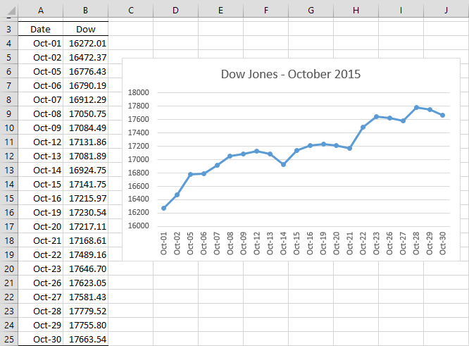
Example 1: Determine whether the Dow Jones closing averages for the month of October 2015, as shown in columns A and B of Figure 1 is a stationary time series.
Figure 1 – Dow Jones Time Series
As you can see from Figure 1, there is an upward trend to the data. This is an indication that the time series is not stationary.
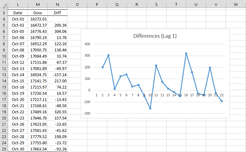
We now take the first differences of the Dow Jones closing averages on consecutive days, as shown in Figure 2.
Figure 2 – Differences of Lag 1
Here cell N5 contains the formula =M5-M4 and similarly for the other cells in column N. This time the chart shows what looks like a random pattern. This is indicative of a stationary time series.
Examples Workbook
Click here to download the Excel workbook with the examples described on this webpage
References
Greene, W. H. (2002) Econometric analysis. 5th Ed. Prentice-Hall
https://www.ctanujit.org/uploads/2/5/3/9/25393293/_econometric_analysis_by_greence.pdf
Gujarati, D. & Porter, D. (2009) Basic econometrics. 5th Ed. McGraw Hill
http://www.uop.edu.pk/ocontents/gujarati_book.pdf
Hamilton, J. D. (1994) Time series analysis. Princeton University Press
https://press.princeton.edu/books/hardcover/9780691042893/time-series-analysis
Wooldridge, J. M. (2009) Introductory econometrics, a modern approach. 5th Ed. South-Western, Cegage Learning
https://cbpbu.ac.in/userfiles/file/2020/STUDY_MAT/ECO/2.pdf


Hi Charles,
A stochastic process (aka a random process) is a collection of random variables ordered by time. This is the “population version” of a time series (which plays the role of a “sample” of a stochastic process).
–> Could you point me in the example 1, What is the collection of random variables ? What is the sample ?
Thanks.
Hello Henry,
The time series is the collection of the data across time taken theoretically from some stochastic process. For each time period, the data element represents a one-element sample from the random variable for that time period.
Charles
Hi,
This is all really helpful, but being new to regression analysis I’m still running into a situation, where I’m not sure how to solve the non-stationarity problem.
I was trying to analyze whether and how strongly is house price index influenced by GDP, demographics (25-44 y.o.) and average homeloan interest rate.
For easier interpretation I logged all the variables and regression results were that all independent variables were significant.
Unfortunately then I found out about time-series having a problem with spurious correlation if the time-series are not stationary. So I checked it with Dickey-Fuller test and indeed, house price index, interest rate and 25-44 y.o. agegroup were non-stationary. Ln(GDP) however was stationary.
What would be the best solution to solve the non-stationarity problem?
You can use such techniques as differencing and detrending. See
https://real-statistics.com/time-series-analysis/stochastic-processes/random-walk/
https://real-statistics.com/time-series-analysis/stochastic-processes/deterministic-trend/
Charles
I’ve tried the differencing and most of my time-series are stationary after first-order differencing (except 25-44 y.o.) according to D-F test. But they all rejected the white noise hypothesis in Ljung-Box white noise test – is that an issue?
Can I use different order differencing in the same model and will this model still be meaningfully interpretable (eg. 1% change in variable causes X% change in dependent variable)?
Madis,
Assuming differencing once is sufficient, you should get white noise. You might need to difference more than once though.
You can use different differencing orders in the same model, but the interpretation will change.
Charles