Random Walk

Basic Concepts

A random walk time series y₁, y₂, …, y_n takes the form

y_i = δ + y_i-1 + ε_i

where

ε_i ∼ N(0, σ²)

cov(ε_i, ε_j) = 0 for i ≠ j

If δ = 0, then the random walk is said to be without drift, while if δ ≠ 0, then the random walk is with drift (i.e. with drift equal to δ).

It is easy to see that for i > 0

It then follows that E[y_i] = y₀ + δi, var(y_i) = σ²i and cov(y_i, y_j) = 0 for i ≠ j. The variance values are not constants but vary with time i, and so this type of time series is not stationary. Also, the mean values are constant only for a random walk without drift.

Note too that since cov(ε_i,ε_j) = 0 for i ≠ j, it follows that

Note that the first difference z_i = y_i – y_i-1 of a random walk is stationary since it takes the form

which is a purely random time series.

Plot

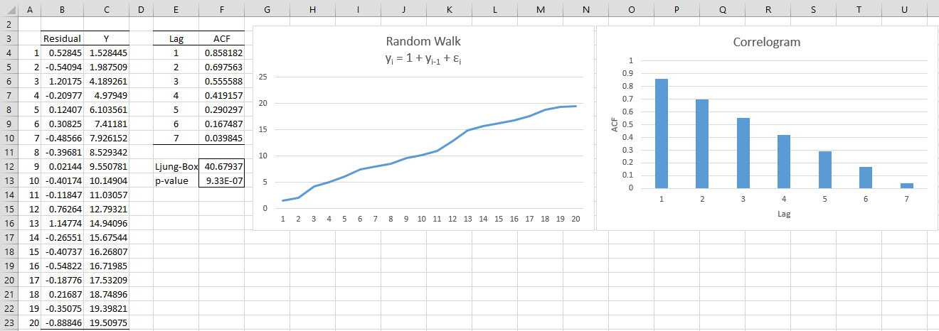
Example 1: Graph the random walk with drift y_i = y_i-1 + ε_i where the ε_i ∼ N(0,.25). (The standard deviation is .5.)

The graph is shown in Figure 1. All the cells in column B contain the formula =NORM.INV(RAND(),0,.5), cell C4 contains the formula =1+B4 and cell C5 contains the formula =1+B5+C4.

As we can see, the graph shows a clear upward trend and the ACF shows a slow descent.

Figure 1 – Random Walk

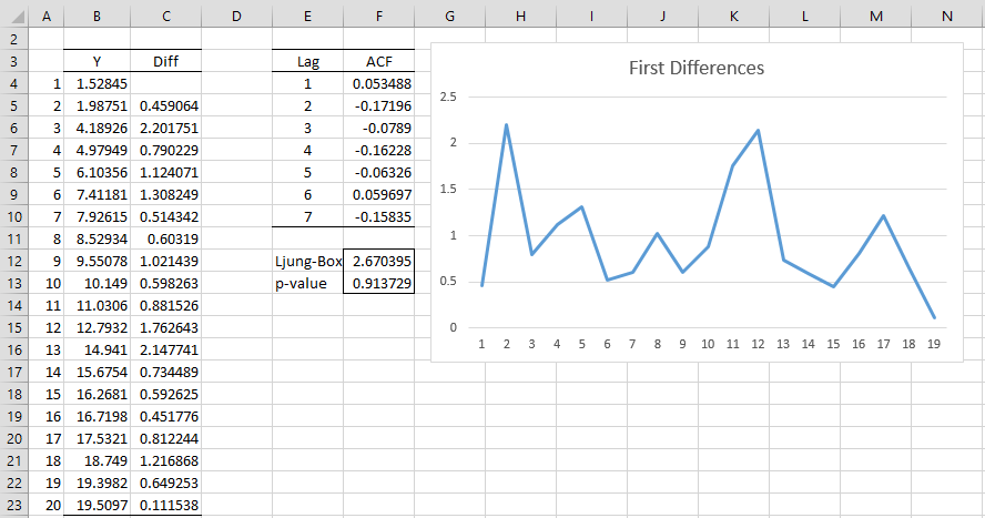
First differences are taken between the y values as shown in Figure 2. E.g. cell C5 contains the formula = B5-B4 (where column B replicates the values in column C from Figure 1). We see from the chart that the trend has been eliminated. We also see from the Ljung-Box test (cell F13) that the ACF values for the first 7 lags are statistically equal to zero, consistent with a purely random process.

Figure 2 – First differences of a random walk

Examples Workbook

Click here to download the Excel workbook with the examples described on this webpage.

References

Greene, W. H. (2002) Econometric analysis. 5th Ed. Prentice-Hall
https://www.ctanujit.org/uploads/2/5/3/9/25393293/_econometric_analysis_by_greence.pdf

Gujarati, D. & Porter, D. (2009) Basic econometrics. 5th Ed. McGraw Hill
http://www.uop.edu.pk/ocontents/gujarati_book.pdf

Hamilton, J. D. (1994) Time series analysis. Princeton University Press
https://press.princeton.edu/books/hardcover/9780691042893/time-series-analysis

Wooldridge, J. M. (2009) Introductory econometrics, a modern approach. 5th Ed. South-Western, Cegage Learning
https://cbpbu.ac.in/userfiles/file/2020/STUDY_MAT/ECO/2.pdf