Purely Random Time Series

A purely random time series y₁, y₂, …, y_n (aka white noise) takes the form

y_i = μ + ε_i

where

ε_i ∼ N(0, σ²)

cov(ε_i, ε_j) = 0 for i ≠ j

Clearly, E[y_i] = μ,  var(y_i) = σ²i and cov(y_i, y_j) = 0 for i ≠ j. Since these values are constants, this type of time series is stationary. Also, note that ρ_h = 0 for all h > 0.

Example

Example 1: Simulate 300 white noise data elements with mean zero.

Using the formula =NORM.S.INV(RAND()) we can generate a sample of 300 white noise elements, as displayed in Figure 1.

Figure 1 – White Noise Simulation

We see that there is a random pattern. Using the techniques described in Autocorrelation Function and Partial Autocorrelation Function we can also calculate ACF and PACF values, as shown in Figure 2.

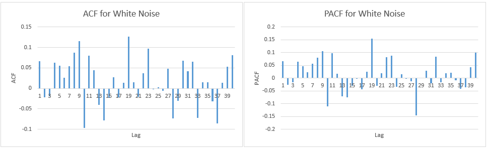
Figure 2 – ACF and PACF for White Noise simulation

Testing

Although the theoretical ACF values are ρ_k = 0 for all k > 0, the sample values r_k won’t necessarily be exactly 0, as we can see from the left side of Figure 2. Based on Property 3 of Autocorrelation Function

r_k ∼ N(0, 1/n)

Since n = 300, a 95% confidence interval for r_k is

0 ± NORM.S.INV(.025)/SQRT(300) = ±0.11316

Figure 2 shows 40 values for r_k. We would expect that about 40(.95) = 2 of these values would be outside the 95% confidence interval. In fact, two ACF values are outside this range, namely r₉ = .11842 and r₁₉ = .13366.

Using the Ljung-Box test, we see that none of the 40 ACF values is significantly different from zero:

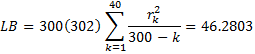
p-value = CHISQ.DIST.RT(46.2803,40) = .229 > .05 = α

We can perform similar tests for the PACF values.

Examples Workbook

Click here to download the Excel workbook with the examples described on this webpage.

References

Greene, W. H. (2002) Econometric analysis. 5th Ed. Prentice-Hall
https://www.ctanujit.org/uploads/2/5/3/9/25393293/_econometric_analysis_by_greence.pdf

Gujarati, D. & Porter, D. (2009) Basic econometrics. 5th Ed. McGraw Hill
http://www.uop.edu.pk/ocontents/gujarati_book.pdf

Hamilton, J. D. (1994) Time series analysis. Princeton University Press
https://press.princeton.edu/books/hardcover/9780691042893/time-series-analysis

Wooldridge, J. M. (2009) Introductory econometrics, a modern approach. 5th Ed. South-Western, Cegage Learning
https://cbpbu.ac.in/userfiles/file/2020/STUDY_MAT/ECO/2.pdf