Partial Autocorrelation Function

Introduction

For regression of y on x₁, x₂, x₃, x₄, the partial correlation between y and x₁ is

This can be calculated as the correlation between the residuals of the regression of y on x₂, x₃, x₄ with the residuals of x₁ on x₂, x₃, x₄.

For a time series, the h^th order partial autocorrelation is the partial correlation of y_i with y_i-h, conditional on y_i-1,…, y_i-h+1, i.e.

The first order partial autocorrelation is therefore the first-order autocorrelation.

Definitions

We can also calculate the partial autocorrelations as in the following alternative definition.

Definition 1: For k > 0, the partial autocorrelation function (PACF) of order k, denoted π_k, of a stochastic process, is defined as the k^th element in the column vector

Here, Γ_k is the k × k autocovariance matrix Γ_k = [v_ij] where v_ij = γ_|i-j| and δ_k is the k × 1 column vector δ_k = [γ_i]. We also define π₀ = 1. We can also define π_ki to be the i^th element in the vector , and so π_k = π_kk.

Provided γ₀ > 0, the partial correlation function of order k is equal to the k^th element in the following column matrix divided by γ₀.

Here, Σ_k is the k × k autocorrelation matrix Σ_k = [ω_ij] where ω_ij = ρ_|i-j| and τ_k is the k × 1 column vector τ_k = [ρ_i].

Note that if γ₀ > 0, then Σ_k and Γ_k are invertible for all m.

The partial autocorrelation function (PACF) of order k, denoted p_k, of a time series, is defined in a similar manner as the last element in the following matrix divided by r₀.

Here R_k is the k × k matrix R_k = [s_ij] where s_ij = r_|i-j| and C_k is the k × 1 column vector C_k = [r_i].

We also define p₀ = 1 and p_ik to be the i^th element in the matrix , and so p_k = p_kk. These values can also be calculated from the autocovariance matrix of the time series in the same manner as described above for stochastic processes.

Observation: Let Y be the k × 1 vector Y = [y₁ y₂ … y_k]^T and Z = [y₁–µ y₂–µ … y_k–µ]^T where µ = E[Y]. Then cov(Y) = E[ZZ^T], which is equal to the k × k autocovariance matrix Γ_k = [v_ij] where v_ij = γ_|i-j|.

Example

Example 1: Calculate PACF for lags 1 to 7 for Example 2 of Autocorrelation Function.

We show the result in Figure 1.

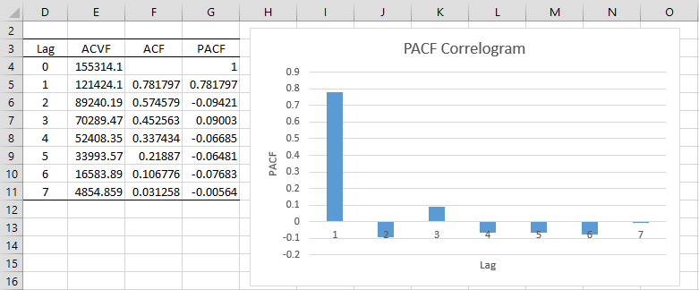
Figure 1 – PACF

We now show how to calculate PACF(4) in Figure 2. The calculations of the other PACF values is similar.

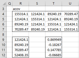
Figure 2 – Calculation of PACF(4)

First, we note that range R4:U7 of Figure 2 contains the autocovariance matrix with lag 4. This is a symmetric matrix, all of whose values come from range E4:E6 of Figure 1. The values on the main diagonal are s₀, the values on the diagonal above and below the main diagonal are s₁. The values on the diagonal two units away are s₂ and finally, the values in the upper right and lower left corners of the matrix are s₃.

Range R9:R12 is identical to range E5:E8. The values in range T9:T12 can now be calculated using the array formula

=MMULT(MINVERSE(R4:U7),R9:R12)

The values in range T9:T12 are the p_i4 values, and so we see that PACF(4) = p₄ = -.06685 (cell T12).

Observations

See Correlogram for information about the standard error and confidence intervals of the p_k, as well as how to create a PACF correlogram that includes the confidence intervals.

We see from the chart in Figure 1, that the PACF values for lags 2, 3, … are close to zero. As can be seen in Partial Autocorrelation for an AR(p) Process, this is typical for a time series derived from an autoregressive process. Note too that we can use Property 3 of Autocorrelation Function to test whether the PACF values for lags 2 and beyond are statistically equal to zero (see Figure 3).

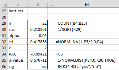
Figure 3 – Bartlett’s test for PACF

The test shows that PACF(2) is not significantly different from zero. Note that, where applicable, we can also use Property 4 and 5 of Autocorrelation Function to test PACF values.

Worksheet Functions

Real Statistics Functions: The Real Statistics Resource Pack supplies the following function where R1 is a column range containing time series data:

PACF(R1, k) – the PACF value at lag k

Real Statistics also provides the following array functions:

ACOV(R1, k) – the autcovariance matrix at lag k

ACORR(R1, k) – the autcorrelation matrix at lag k

Non-negative definite

Property 1: The autocovariance matrix is non-negative definite (See Positive Definite Matrices)

Proof: Let Y = [y₁ y₂ … y_k]^T and let Γ be the k × k autocovariance matrix Γ = [v_ij] where v_ij = γ_|i-j| . As we observed previously, Γ = E[ZZ^T].

Now let X be any k × 1 vector. Then

which completes the proof.

Examples Workbook

Click here to download the Excel workbook with the examples described on this webpage.

References

Greene, W. H. (2002) Econometric analysis. 5th Ed. Prentice-Hall
https://www.scirp.org/(S(351jmbntvnsjt1aadkposzje))/reference/referencespapers.aspx?referenceid=1243286

Gujarati, D. & Porter, D. (2009) Basic econometrics. 5th Ed. McGraw Hill
http://www.uop.edu.pk/ocontents/gujarati_book.pdf

Hamilton, J. D. (1994) Time series analysis. Princeton University Press
https://press.princeton.edu/books/hardcover/9780691042893/time-series-analysis

Wooldridge, J. M. (2009) Introductory econometrics, a modern approach. 5th Ed. South-Western, Cegage Learning
https://cbpbu.ac.in/userfiles/file/2020/STUDY_MAT/ECO/2.pdf