Example
Example 1: Create a SARIMA(1,1,1) ⨯ (1,1,1)4 model for Amazon’s quarterly revenues shown in Figure 1 and create a forecast based on this model for the four quarters starting in Q3 2017.
Note that the range A3:B33 contains all the data, where the second half of the data is repeated in columns D and E (so that it is easier to display in the figure).
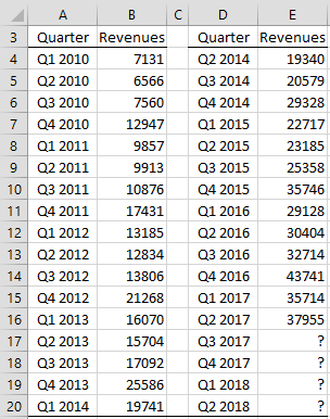
Figure 1 – Amazon Revenues
We start by creating a plot of the time series data by highlighting the range B4:B33 and then selecting Insert > Charts|Line. After making a few modifications we obtain the result shown in Figure 2.

Figure 2 – Plot of Amazon Revenues
Differencing
We see from the chart that there is an upward trend and there is seasonality. We next try to remove the trend and seasonality by differencing, as shown on the left side of Figure 3.
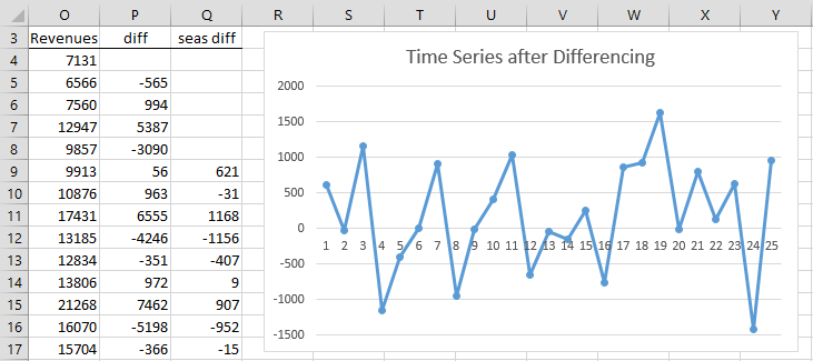
Figure 3 – Ordinary and seasonal differencing
The original revenue data is repeated in range O3:O33 (with only the first 14 data elements visible in the figure). Column P contains the detrended data where cell P5 contains the formula =O5-O4, and similarly for the other cells in column P. Column Q removes the seasonality from the data in column P. We do this by inserting the formula =P9-P5 in cell Q9, highlighting the range Q9:Q33 and pressing the key sequence Ctrl-D.
We next plot the data in column Q as shown on the right side of Figure 3. This time the plot looks like it comes from a stationary time series, although we would need to perform a unit root test to confirm this.
Residuals
Figure 4 shows how to calculate the residuals for the SARIMA model of this time series in terms of the coefficients (only the first 8 of the time series entries in AG3:AI28 are displayed).
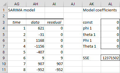
Figure 4 – Calculation of residuals
The values in range AH4:AH28 are copied from Q9:Q33 of Figure 3. As we saw SARIMA Models, the residuals of this time series can be calculated using the formula
![]()
To calculate εi we need to know the values of εi-1, εi-4, εi-5. Thus we arbitrarily set the values of the first five residuals equal to zero and use the above formula to calculate ε6 (cell AI9). We can do this in Excel using the following worksheet formula
=AH9-AL$3-AL$4*AH8-AL$6*AH5+AL$4*AL$6*AH4-AL$5*AI8-AL$7*AI5-AL$5*AL$7*AI4
Next, we highlight range AI9:AI28 and press Ctrl-D to fill in the values of all the rest of the residuals. Since we initially set all the coefficients to zero, the residuals initially all take the same value as the data.
Using Solver
Our goal is to find coefficients that minimize the sum of the squares of the residuals (SSE). We accomplish this by using Excel’s Solver. The value of SSE is calculated in cell AL9 using the formula =SUMSQ(AI9:AI28).
Select Data > Analysis|Solver and fill in the dialog box that appears as shown in Figure 5.
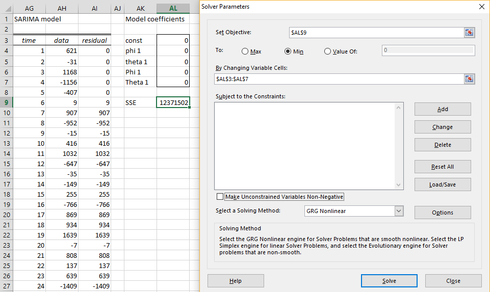
Figure 5 – Solver dialog box
After clicking on the Solve button, the results shown in Figure 6 appear.
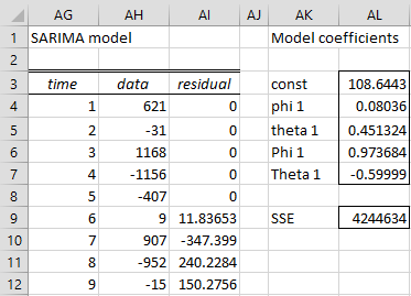
Figure 6 – Solver results
As you can see, the residual values shown in column AI change and the new SSE value of 4,244,634 is much less than the initial value shown in Figure 4.
Examples Workbook
Click here to download the Excel workbook with the examples described on this webpage.
References
Greene, W. H. (2002) Econometric analysis. 5th Ed. Prentice-Hall
https://www.ctanujit.org/uploads/2/5/3/9/25393293/_econometric_analysis_by_greence.pdf
Gujarati, D. & Porter, D. (2009) Basic econometrics. 5th Ed. McGraw Hill
http://www.uop.edu.pk/ocontents/gujarati_book.pdf
Hamilton, J. D. (1994) Time series analysis. Princeton University Press
https://press.princeton.edu/books/hardcover/9780691042893/time-series-analysis
Wooldridge, J. M. (2009) Introductory econometrics, a modern approach. 5th Ed. South-Western, Cegage Learning
https://cbpbu.ac.in/userfiles/file/2020/STUDY_MAT/ECO/2.pdf
Im performing a forecasting model where im trying to run the SARIMA model to forecast eps. When i tried your method the coefficients that i im getting are all the of same values
Hello Vidyesh,
If you email me an Excel sheet with your data and results I will try to figure out what is going wrong.
Charles
I follow your steps in Excel but the value were different after run the Solver. Any idea why it happened?
Can you email me an example of where this happens?
Charles
Hello Charles,
Sure, can I have your email?
See Contact Us
Charles
How can one rate SARIMA’s forecasting ability against other models, e.g., regression, Holt-Winters, etc., when there is no ability to compare forecast errors, whether RMSE, etc.?
Hello Mark,
I don’t know a way to compare forecast models without having some measure of forecast errors.
Presumably, you have some data to use to create the forecast model(s). You can use most of the data to create the model(s) and the rest to test the accuracy of the model(s).
Charles
Charles
As usual, I failed to pose my question with enough clarity.
I have a data set – histrical Amazon quarterly revenue. I can create a 4 quarter forecast using different models. One of thos models is a SARIMA model. Another might be a linear regression model, with time trend and seasonal dummy variables as the independent variables. I could use a Holt-Winters model, but you get the picture. The forecast results I get are all reasonably close to each other, but I am looking for metric – RMSE, e.g. to compare the results. How do you get the RMSE for SARIMA in back-transformed space?
Hi Mark,
As I said in my previous response, I don’t know how you get a back-transformed metric, but I proposed another approach. Suppose you have 20 quarters of data and want to forecast 4 quarters ahead. I don’t know how to compare the forecast of the next 4 quarters, but I can use say 16 quarters of the existing data to build the models that I want to compare. I can then use these models to forecast the next 4 quarters, but since I have the observed data for these 4 quarters, I can calculate the RMSE (or other metrics) for each of the models and compare the results.
Charles
Charles
So, with a SARIMA model one can only compare the 4 quarter forecast with the actual results for those quarters. That is, there is no way to “forecast” the 16 quarters and compare them by way of RMSE to the actual 16 quarters?
If so, that’s too bad as most of the time I am forecasting “but for” revenue and have no actual revenue to compare it to. Therefore, I default to RMSE of “forecasted” past data with actual past data.
Mark,
Unfortunately, this is the case. See the following for more details.
https://otexts.com/fpp2/accuracy.html
Charles
Charles
Now I get it. While familiar with the concept of hold-back forecasting, It did not dawn on me to use it to test the accuracy of various models when RMSE could not be applied to past history, as in a SARIMA model.
Thanks for the tip and your patience.
Mark
Why P9-P5?
The seasonality is 4. P5 is the first cell in the diff column. 4 cells later is cell P9.
Charles