We now show how to simplify the process of creating a SARIMA model by using Real Statistics capabilities.
Worksheet Functions
Real Statistics Functions: The Real Statistics Resource Pack supplies the following array functions:
ADIFF(R1, d, D, per): returns a column array that corresponds to the time series data in R1 after ordinary differencing d times and seasonal differencing D times based on a seasonal period of per.
This function is an extension to the version described in ARIMA Differencing.
SARMA_RES(R1, Rar, Rma, Rsa, Rsm, per, cons): returns a column array with the residuals that correspond to the time series data in the column array R1 based on a SARMA model with AR coefficients in Rar, MA coefficients in Rma, seasonal AR coefficients in Rsa, seasonal MA coefficients in Rsm, the constant coefficient in cons and the seasonal period per.
Prediction functions
SARMA_PRED(R1, Rar, Rma, Rsa, Rsm, per, cons, f): returns a column array with the predicted values that correspond to the time series data in the column array R1 plus the next f forecast values based on a SARMA model with AR coefficients in Rar, MA coefficients in Rma, seasonal AR coefficients in Rsa, seasonal MA coefficients in Rsm, the constant coefficient in cons and the seasonal period per. If f is omitted then the highlighted (output) range is filled with forecasted values (i.e. f is set equal to the number of rows in the highlighted range minus the number of rows in R1).
SARIMA_PRED(R0, R1, d, D, per): returns a column array with the forecasted values for the SARIMA(p, d, q) ⨯(P, D, Q)per model of the time series data in R1 that correspond to the forecast values in R0 for the SARMA(p, q) ⨯(P, Q)per model.
All the above arrays are column arrays. Any of the Rar, Rma, Rsa, Rsm arrays may be omitted, although at least one of these can’t be omitted. per defaults to 12 and cons defaults to 0 (i.e. no constant).
Example
The above functions make it easier to create a SARIMA model and forecast. We can illustrate this for Example 1 of SARIMA Model Example which shows how to create a SARIMA(1, 1, 1) ⨯ (1, 1, 1)4 model and forecast, using the following formulas:
=ADIFF(B4:B33,1,1,4) to create the time series in range AH4:AH28 of Figure 4 of SARIMA Model Example
=SARMA_RES(AH4:AH28,AL4,AL5,AL6,AL7,4,AL3) to create the array of residuals in range AI4:AI28 of Figure 4 of SARIMA Model Example
=SARMA_PRED(AH4:AH28,AL4,AL5,AL6,AL7,4,AL3) to create an array of predicted values that take the values in the array AH4:AH32 – AI4:AI32 of Figure 4 of SARIMA Model Example. In particular, the last 4 of these values are those found in range AH29:AH32.
=SARIMA_PRED(AH29:AH32,B4:B33,1,1,4) to create the array of forecast values shown in range AO10:AO13 of Figure 3 of SARIMA Forecast Example.
Data Analysis Tool
Real Statistics Data Analysis Tool: The Real Statistics Resource Pack provides the Seasonal Arima (Sarima) data analysis tool which creates a SARIMA model and forecast.
To perform the analysis for Example 1 of SARIMA Model Example, press Ctrl-m and choose Seasonal Arima (Sarima) from the Time S tab (or from the Time Series dialog box if using the original user interface). Now fill in the dialog box that appears as shown in Figure 1.
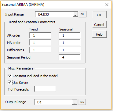
Figure 1 – SARIMA dialog box
If you leave the # of Forecasts field blank, then its value defaults to the value in the Seasonal Period field. If that field is blank then no seasonality is used in the model and # of Forecasts defaults to 5.
Output
After clicking on the OK button, the output shown in Figures 2 and 3 is displayed (only the first 24 rows of the output in Figure 2 and the first 20 rows in Figure 3 are displayed).
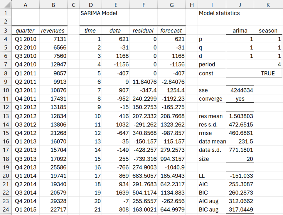
Figure 2 – SARIMA output (part 1)
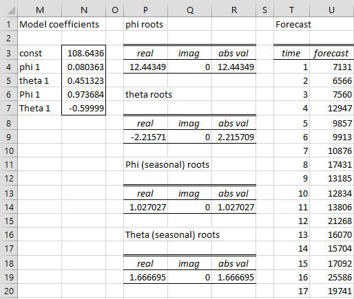
Figure 3 – SARIMA output (part 2)
Most of the values are produced using the Real Statistics functions described above. The formulas used for the descriptive statistics in range J13:J24 and coefficient roots in columns P, Q and R are similar to those used for the corresponding values in the Arima data analysis tool.
Forecast
The lower portion of the output, which contains the forecast, is shown in Figure 4. The values in columns D, E, F and G are the continuation of these columns from Figure 2 and the values in columns T and U are the continuation of these columns from Figure 3.
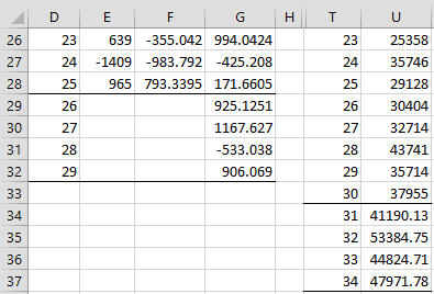
Figure 4 – SARIMA forecast output
Range G29:G32 contains the four-quarter forecast for the differenced time series, while range U34:U37 contains the corresponding four-quarter forecast for the revenues for the period Q3 2017 through Q2 2018.
Levenberg-Marquardt approach
For this example, we chose to use the Solver approach to estimating the SARIMA coefficients. The default is to use the Levenberg-Marquardt approach. This is accomplished by leaving the Solver option unchecked in Figure 1. In this case, the output is similar to that described above, except that now the output in Figure 5 is included, which is useful in that it provides the standard errors of the coefficients and the t-tests that determine which coefficients are significantly different from zero.
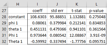
Figure 5 – SARIMA coefficients
The output in range H27:L32 of Figure 5 is produced by the array formula
=SARIMA_PARAM(A1:A30,I4,I5,I6,J7,J4,J5,J6,J8)
More Worksheet Functions
Real Statistics Functions: The Real Statistics Resource Pack supplies the following array functions:
SARIMA_COEFF(R1, ar, ma, diff, per, sar, sma, sdiff, con, lab): returns an array with two columns, the first column of which contains the SARIMA coefficients (in the order constant term, phi coefficients, theta coefficients, Phi coefficients, Theta coefficients) and the second column contains the corresponding standard errors. If lab = TRUE (default FALSE) then a column of labels is appended to the output.
SARIMA_PARAM(R1, ar, ma, diff, per, sar, sma, sdiff, con): returns an array with four columns, the first column of which contains the SARIMA coefficients (in the order constant term, phi coefficients, theta coefficients, Phi coefficients, Theta coefficients) and the remaining columns contain the corresponding standard errors, t statistics and p-values.
Here, the parameters are ar = p, ma = q, diff = d, per = m, sar = P, sma = Q, sdiff = D for a (p, d, q) × (P, D, Q)m SARIMA model. con = TRUE (default) if a constant term is included.
Examples Workbook
Click here to download the Excel workbook with the examples described on this webpage.
References
Greene, W. H. (2002) Econometric analysis. 5th Ed. Prentice-Hall
https://www.ctanujit.org/uploads/2/5/3/9/25393293/_econometric_analysis_by_greence.pdf
Gujarati, D. & Porter, D. (2009) Basic econometrics. 5th Ed. McGraw Hill
http://www.uop.edu.pk/ocontents/gujarati_book.pdf
Hamilton, J. D. (1994) Time series analysis. Princeton University Press
https://press.princeton.edu/books/hardcover/9780691042893/time-series-analysis
Wooldridge, J. M. (2009) Introductory econometrics, a modern approach. 5th Ed. South-Western, Cegage Learning
https://cbpbu.ac.in/userfiles/file/2020/STUDY_MAT/ECO/2.pdf
Hi Charles,
Your site is incredible and SO helpful to my forecasting job, thank you!!!
I am forecasting a product in excel, recorded in monthly sales.
I have entered:
AR order 1,1
MA order 1,1
Differences 1,1
What Seasonal Period number should I use?
When I try to enter 12, I get the error “Input must have at least 2p+q+d+P+Q+(P+D)*m+2 rows of data (one less if no constant)
I have tried seasonal period of 4 & 6, but neither forecast looks great. Am I doing something wrong?
Hello Penn,
Thank you for your kind words about the Real Statistics website.
It looks like you don’t have enough data. The model can’t estimate the coefficients based on your model specification with this amount of data.
This is what the 2p+q+d+P+Q+(P+D)*m+2 rows of data refers to.
Charles
Hello Charles,
I am looking for the Levenberg-Marquardt method in Excel to optimize a model with more than 10 parameters. Can I use the SARIMA functions outside a SARIMA model?
Thank you.
Felix
Hello Felix,
Real Statistics uses the Levenberg-Marquardt method in Excel for ARIMA and SARIMA but it won’t necessarily be useful outside SARIMA or ARIMA.
Charles
Hi, Charles,
On the SARIMA feature of Real Statistics, I think the statistic “sqrt mse”, the RMSE fit statistic, is actually the MSE instead. On the “SARIMA” tab of the example workbook, the SSE is computed as 4244634.32. The “size” is 20. Therefore, the MSE is 4244634.32/20 = 212231.716. The RMSE should therefore be sqrt(212231.716) = 460.686.
Am I correct in my thinking?
Hello Kevin,
Yes, you are correct in your thinking. I will use RMSE = 460.686.
Thanks for your help.
Charles