Calculating MA Coefficients using ACF

Introduction

If we know (or assume) that a time series can be fit by an MA(q) process, then we need to figure out the value of the parameters μ, σ², q, θ₁, …, θ_q.

The initial approach to determining the value for q is to look at the ACF values for the time series under consideration. Since we know that for an MA(q) process, ρ_k = 0 for all k > q, we seek the first value for q where ACF(q) is approximately zero. We will refine this approach in Comparing ARIMA Models.

We next turn our attention to finding the other parameters that provide the best fit for the data.

MA(1) Properties

We start by looking at an MA(1) process  y_i = μ + ε_i + θ₁ε_i-1 . 

Property 1: The mean is μ.

Property 2: The variance is

Property 3: The autocorrelation function is

We start by using the mean of the time series as μ. We then subtract this value from all the time series values to get a zero mean time series. We then calculate the variance s² and r = ACF(1) of the time series. We can solve for θ₁ using the equation

which is equivalent to the quadratic equation

and has the solutions

Actually θ₁ above is really the estimated value of θ₁ which typically has a hat over it. These solutions are real provided |r| < .5. It turns out that for large values of n

where

Also, note that

Example

Example 1: Assuming that the time series in range C4:C203 of Figure 1 fits an MA(1) process (only the first 10 of 200 values are shown), find the values of μ, σ², θ₁ for the MA(1) process.

We actually created the time series using the MA(1) process y_i = ε_i – .4ε_i-1 with σ² = .25. Thus, we entered the formula =NORM.INV(RAND(),0,.5) in all the cells in range B4:B203 and placed the formula =B4 in cell C4 and the formula =B5-.4*B4 in cell C5. We then highlighted range C5:C203 and pressed Ctrl-D.

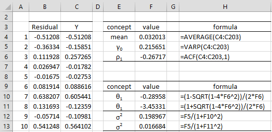
Figure 1 – Calculating MA(1) parameters

We now calculate the mean (cell F4), variance (cell F5) and autocorrelation from the time series as shown in the upper right-hand side of Figure 1. From these values, we calculate two possible values for θ₁, namely -0.28958 and -3.45331. Note that these values are reciprocals of one another. Only the value θ₁ = -0.28958 yields an invertible MA(1) process since |θ₁| < 1. In this case, we see that σ² = 0.198967.

The result is an estimate of the MA(1) process, namely

with an estimate of 0.198967 for the variance of the ε_i. Using a one-sample t-test, we can see that the mean is not significantly different from zero (t = .97, p-value = .33, 2 tailed test).

Confidence Interval

We can compute a somewhat crude 95% confidence range for θ₁ based on the normal approximation, as shown in Figure 2.

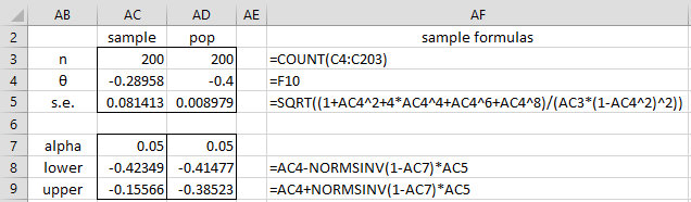
Figure 2 – Confidence interval

If we knew the real value of θ₁ the confidence interval would be as shown in column AD of Figure 2. Since we don’t know the actual value of θ₁ we have to make do with the values estimated in Figure 1 when calculating the standard error (as shown in column AC of Figure 2). Thus, we see that the real value lies in the interval (-.42349, -.15566) with 95% confidence.

Observation: In the above example we used a sample with 200 elements. When we repeated the same analysis with a sample of 1,000 elements we got the following estimates, which are closer to the original MA(1) process parameters:

with σ² = 0.23683. The 95% confidence interval for θ₁ also narrowed to (-.446, -.311).

We can obtain better estimates using other techniques, as shown in Calculating MA(q) Coefficients using Solver.

Estimate of σ²

When using the method of moments approach to estimating the MA(q) coefficients, we can estimate the variance of the error terms via the following formula:

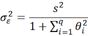
where s² is the variance for the time series

References

Greene, W. H. (2002) Econometric analysis. 5th Ed. Prentice-Hall
https://www.scirp.org/(S(351jmbntvnsjt1aadkposzje))/reference/referencespapers.aspx?referenceid=1243286

Gujarati, D. & Porter, D. (2009) Basic econometrics. 5th Ed. McGraw Hill
http://www.uop.edu.pk/ocontents/gujarati_book.pdf

Hamilton, J. D. (1994) Time series analysis. Princeton University Press
https://press.princeton.edu/books/hardcover/9780691042893/time-series-analysis

Wooldridge, J. M. (2009) Introductory econometrics, a modern approach. 5th Ed. South-Western, Cegage Learning
https://cbpbu.ac.in/userfiles/file/2020/STUDY_MAT/ECO/2.pdf