We now show how to use Excel’s Solver to calculate the parameters that best fit an MA(q) process to some empirical time series data. This is based on the assumption that the data does indeed fit an MA(q) process for some specific value of q.
MA(1) Example
Example 1: Repeat Example 1 of Calculating MA Coefficients using ACF using Solver.
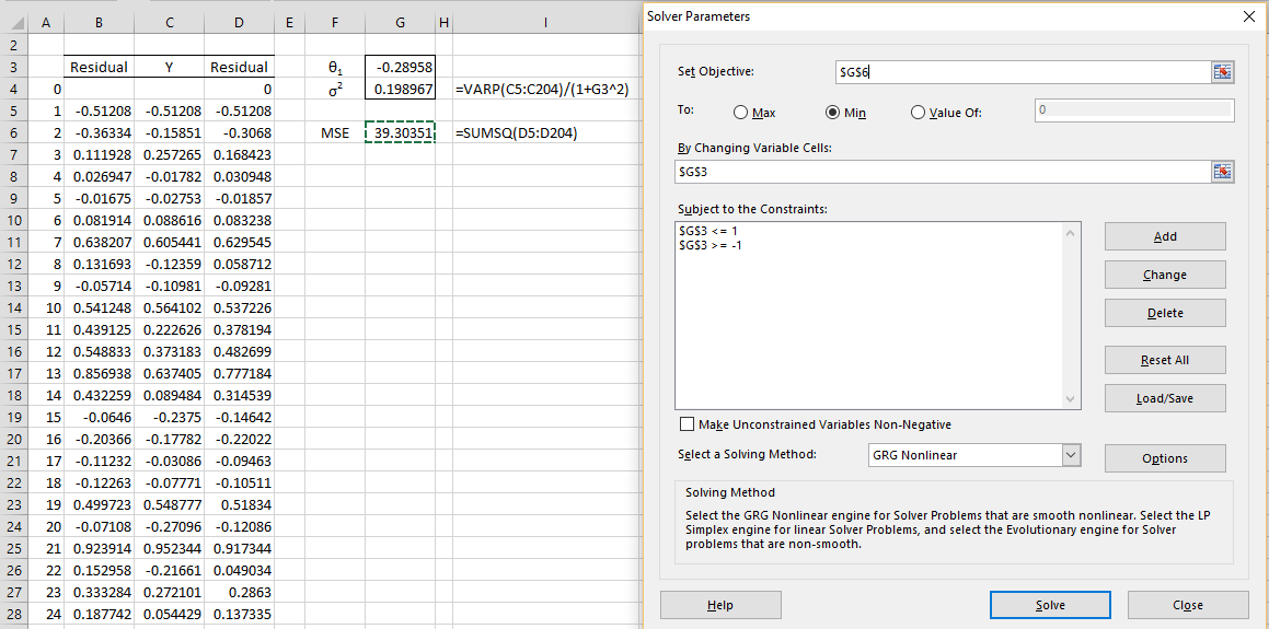
We create a 200 element time series by simulating the MA(1) process yi = εi – .4εi-1 with σ2 = .25. The values in the time series are shown in range C4:C203 of Figure 1.
Our goal is to fit this data to an MA(1) process of the form yi = μ + εi + θ1εi-1. We will ignore the fact that the time series was originally derived from a simulation of an MA(1) process.
Figure 1 – Using Solver to fit an MA(1) process
Motivation
As we have done many times, we use the mean of the time series to provide an estimate of the mean of the process. Specifically, the estimate of μ = AVERAGE(C4:C203) = .03293, which we have noted previously is not significantly different from zero.
We can now either subtract off this value for the mean from the y values in column C or simply assume that the mean is zero, and proceed assuming that μ = 0, which is what we will do here.
Since yi = εi + θ1εi-1, it follows that εi = yi – θ1εi-1. Thus, for any estimated value of θ1, we can calculate the values of the εi for i > 1 based on the data values in the time series and the assumption that the initial residual value is zero, i.e. ε0 = 0.
Set-up
We accomplish this by placing 0 in cell D4 of Figure 1. Next, we insert the formula =C5-$G$3*D4 in cell D5, highlight the range D5:D203 and press Ctrl-D.
By Property 2 of Moving Average Processes Basic Concepts
and so an estimate for σ2 can be calculated from the estimate for θ1 using the formula VAR.P(C5:C204) or VARP(C5:C204) as an estimate for var(yi). This is the formula in cell G4 of Figure 1.
We use as an initial guess for the value of θ1 the value calculated by using the ACF estimate from Example 1 of Calculating MA Coefficients using ACF, namely 0.28958, although we could simply use 0. As usual, we will use Solver to minimize the mean squared error (MSE), which is simply the sum of the squares of the εi values, as shown by the formula in cell G6 of Figure 1.
We now select Data > Analysis|Solver which brings up the dialog box shown on the right side of Figure 1. Solver will attempt to minimize MSE (cell G6) by changing the value of θ1 (cell G3). Note that since we want to restrict θ1 to have an absolute value less than 1, we add the constraints shown in the dialog box. We could also add a constraint to ensure that σ2 > 0, although this is not necessary since the formula in cell G4 already creates this constraint (provided all the data elements in column C are not equal).
Results
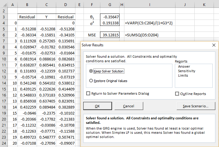
When we click on the Solve button, the results shown in Figure 2 appear.
Figure 2 – Solver output for MA(1) process
We see that MSE is minimized when θ1 = -0.35909, a value that is closer to the original value than the result from Example 1 of Calculating MA Coefficients using ACF.
Finally, we should make sure that the residual values in column D are consistent with white noise. We see this by using the Ljung-Box test or looking at the Correlogram, as shown in Figure 3.
Figure 3 – Check that residuals are white noise
MA(2) Example
Example 2: Repeat Example 1 trying to fit the data with an MA(2) process.
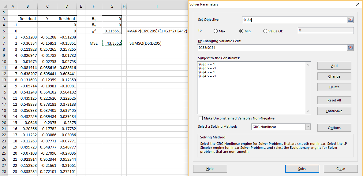
The approach is the same, except that this time, we calculate the residuals using the formula εi = yi – θ1εi-1 – θ2εi-2, and assume that ε0 = ε-1 = 0. E.g., this is captured in Excel by using the formula =C6-$G$3*D5-G$4*D4 in cell D6 and similarly for the other cells in column D.
The setup for Solver is shown in Figure 4 using initial guesses of θ1 = θ2 = 0.
Figure 4 – Using Solver to fit an MA(2) process
The output is shown in Figure 5.
Figure 5 – Solver output for MA(2) process
This results in the MA(2) process
yi = εi – 0.31991εi-1 – 0.06596εi-2
with σ2 = 0.194861.
In Comparing ARIMA Models we discuss how to determine which model is a better fit, the MA(1) process from Example 1 or the MA(2) process from Example 2. We also show how to use this model for forecasting in ARIMA Forecasting.
Examples Workbook
Click here to download the Excel workbook with the examples described on this webpage.
References
Borah, B. (2024) Understanding moving average (MA) models in time series analysis
https://medium.com/@bhargavborah020/understanding-moving-average-ma-models-in-time-series-analysis-d18e443f15cc
Geeks for Geeks (2024) Understanding the moving average (MA) in time series data
https://www.geeksforgeeks.org/understanding-the-moving-average-ma-in-time-series-data/
Hyndman, R. J., Athanasopoulos, G. (2018) Moving average models. Forecasting: principles and practice
https://otexts.com/fpp2/MA.html
Hamilton, J. D. (1994) Time series analysis. Princeton University Press
https://press.princeton.edu/books/hardcover/9780691042893/time-series-analysis


Hi Charles,
I’ve really appreciated this post so far in my trying to learn time series analysis.
Could you pls help me with a couple of simple questions on the Excel sheet that you show in Fig 1 for Example 1:
1) I get the correct values in D5 and D6, 0.51208 and 0.3068, with the formula =C5-$D$3*D4 starting in cell D5. But the value I get for D7 using the very same formula, =C7-$G$3*D6 is different, 0.3461, not the 0.168423 shown.
2) What are the values showing in column B? The instructions to not appear to make use of them at all.
Hello Bong,
1. The formula in D5 is =C5-$G$3*D4. For D7, we get D7 = C7-$G$3*D6 = .257265 – (-.35647)*(-.34105) = .257265 – .35647*.34105 = .257265 – .121574 = .135691 (from Figure 2).
2. The way the example works is that I start with a series of residuals ε_t (in column B). I then use these to create a time series
y_t = ε_t + .4ε_t-1 (in column C). I then proceeded to fit this time series to an MA(1) process. Given how we created the time series we expect that the coefficient for the MA(1) process would be -.4 (or at least reasonably close).
Charles
I appreciate your taking the time to respond Charles. God bless
could you please help me to understand how to calculate the θ1 (cell G3)?
thank you so much
Omega-1 is estimated iteratively using Excel’s Solver capability. The objective is to find the value of Omega-3 that minimizes the MSE value. See the following webpage regarding how to use Solver.
https://www.real-statistics.com/chi-square-and-f-distributions/two-sample-hypothesis-testing-comparing-variances/
Charles
Hi! Your site really helped me. But I have one question that I can’t find an answer to. In MA(1) model the zero residual in your example is 0, but programs like Gretl, SPSS somehow calculate it. Because of this, the divergence in the found coefficients. Thanks
Hello John,
Are you referring to the zero residual for the first time period?
There are various ways of assuming a value for this first residual, but none of these techniques is especially useful in my opinion. With enough data, the results should be similar anyway.
Charles
I try to calculate coefficient of MA(1) model using solver and that’s what I got (screenshot): https://www.dropbox.com/s/7m9fkjre1moap2m/Screenshot_4.png?dl=0
The coefficients are different, all due to the fact that there is no zero error. I searched for a lot of time on the Internet for an answer on how to calculate it (formula). The only thing I found was a reverse forecast, which is already based on aligned data on the model. e0 = (Xt-μ-e1) / Θ. And this formula is not suitable for calculation (circular link in Excel).
Thank you for your reply! And if you help solve this mystery, I will be very grateful to you !!! (sorry for the link, but I think it shows that it refers to a picture and is safe)
Hello John,
I really don’t understand the mystery that you are referencing.
In any case, I make the following observations:
1. The results from Real Statistics and Gretl are actually pretty similar. I was able to duplicate the results in your screenshot. The Gretl theta value with constant zero yields SSE a little larger than the value obtained by Real Statistics. This should mean that the Real Statistics value is a little better.
2. If you look at the model with a non-zero constant value, you will see that the constant is significantly different from zero (p = .0067) and so should be included in the model unless there is a reason to do otherwise.
Charles
I want to say that I am very learning from your site, But I do not understand Moving average model.
could you please help me to understand how to calculate the White noise?
thank you so much
Mustafa
Hi Mustafa,
See the following re white noise:
https://real-statistics.com/time-series-analysis/stochastic-processes/purely-random-time-series/
Charles