Suppose that we have two forecasts f1, …, fn and g1, …, gn for a time series if y1, …, yn and we want to see which forecast is better, in the sense of it having better predictive accuracy. The obvious approach is to select the forecast that has the smaller error measurement based on one of the error measurements described in Forecasting Errors. But we need to go one step further and determine whether this difference is significant (for predictive purposes) or simply due to the specific choice of data values in the sample.
Basic Concepts
We use the Diebold-Mariano test to determine whether the two forecasts are significantly different. Let ei and ri be the residuals for the two forecasts, i.e.
and let di be defined as one of the following (or other similar measurements)
The time series di is called the loss-differential. Clearly, the first of these formulas is related to the MSE error statistic and the second is related to the MAE error statistic. We now define
For n > k ≥ 1, define
As described in Autocorrelation Function γk is the autcovariance at lag k.
For h ≥ 1, define the Diebold-Mariano statistic as follows:
It is generally sufficient to use the value h = n1/3 + 1.
Under the assumption that μ = 0 (the null hypothesis), DM follows a standard normal distribution:
DM ∼ N(0, 1)
Thus, there is a significant difference between the forecasts if |DM| > zcrit where zcrit is the two-tailed critical value for the standard normal distribution; i.e.
zcrit = NORM.S.DIST(1–α/2, TRUE)
The key assumption for using the Diebold-Mariano test is that the loss differential time series di is stationary (see Stationary Time Series).
Example
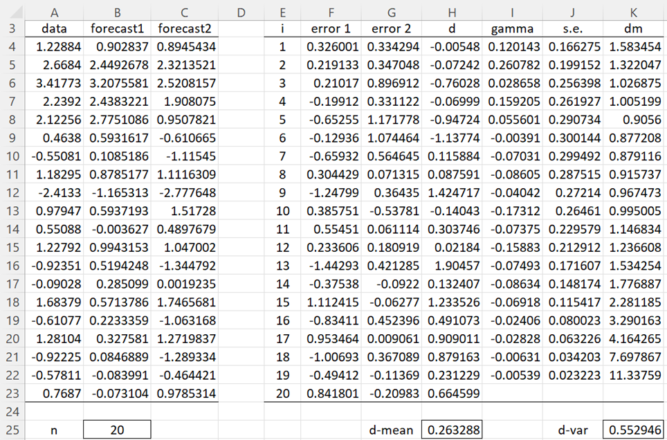
Example 1: Use the Diebold-Mariano test to determine whether there is a significant difference in the forecast in columns B and C of Figure 1 for the data in column A.
Figure 1 – Diebold-Mariano Test
Calculations
We begin by calculating the residuals for the 20 data elements based on the two forecasts (columns F and G). E.g. cell F4 contains the formula =A4-B4 and cell G4 contains =A4-C4. From these values we can calculate the loss-differentials in column H. E.g. cell H4 contains =F4^2-G4^2. We can now calculate the mean and variance of the di time series via the formulas =AVERAGE(H4:H23) and =VAR.P(H4:H23), as shown in cells H25 and K25.
The γi values can now be calculated as shown in column I. E.g. cell I4 contains the array formula
=SUMPRODUCT(H5:H$23-H$25,OFFSET(H$4:H$23,0,0,E$23-E4)-H$25)/E$23
Alternatively, cell I4 can be calculated using the formula =ACVF(H$4:H$23,E4), as described in Autocorrelation Function. The standard errors (column J) and Diebold-Mariano statistics (column K) can next be calculated. E.g. cell J4 contains the formula =SQRT(J25/E23), cell J5 contains =SQRT((J$25+2*SUMPRODUCT(I$4:I4))/E$23) (and similarly for the other cells in column J) and cell K4 contains the formula =G$25/J4.
Conclusions
We can read out the DM statistics values from column K. E.g. the DM statistic for order h = 4 is 1.005199, as shown in cell K7. Note that since h = n1/3 + 1 = 201/3 + 1 = 3.7, h = 4 seems to be a good order value to use. Now since p-value = 2*(1-NORM.S.DIST(K7,TRUE)) = .3148 > .05 = α, we conclude there is no significant difference between the two forecasts.
Forecast Plot
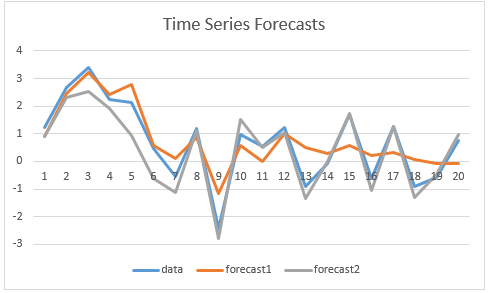
In Figure 2, we plot the two forecasts for the data in column A, and so you can judge for yourself whether the chart is consistent with the results from the Diebold-Mariano test.
Figure 2 – Comparing time series forecasts
HLN Test
The Diebold-Mariano test tends to reject the null hypothesis too often for small samples. A better test is the Harvey, Leybourne, and Newbold (HLN) test, which is based on the following:
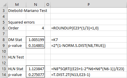
Especially since for Example 1 we have a small sample, we use the HLN test as shown in Figure 3. Once again, we see that there is no significant difference between the forecasts.
Figure 3 – HLN Test
Real Statistic Support
Click here for information about Real Statistics support for the Diebold-Mariano and HLN tests.
Examples Workbook
Click here to download the Excel workbook with the examples described on this webpage.
References
Diebold, F. X. and Mariano, R. S. (1995). Comparing predictive accuracy. Journal of Business and Economic Statistics, 13: 253-63.
https://www.sas.upenn.edu/~fdiebold/papers/paper68/pa.dm.pdf
Harvey, D., S. Leybourne, and P. Newbold. (1997). Testing the equality of prediction mean squared errors. International Journal of Forecasting, 13: 281-91.
Triacca, U. (2016) Lesson 19: comparing predictive accuracy of two forecasts: the Diebold-Mariano test.
No longer available online
Ibisevic, S. (2017) Diebold-Mariano test statistic. MathWorks
https://it.mathworks.com/matlabcentral/fileexchange/33979-diebold-mariano-test-statistic?focused=7267180&tab=function
Diebold, F. X. (2012) Comparing predictive accuracy, twenty years later: a personal perspective on the use and abuse of Diebold-Mariano tests
https://www.nber.org/system/files/working_papers/w18391/w18391.pdf


Dr Zaionitz buenas tardes, porque razón la prueba de Timmermman, no se puede aplicar o mejor no se puede obtener un valor p, si la serie de tiempo y sus pronósticos so positivos?
Gracias
Dr. Zaionitz, good afternoon. For what reason can the Timmermans test not be applied, or more precisely, why can a p-value not be obtained, if the time series and its forecasts are positive? Thank you.
Hello Gerardo,
Sorry, but I don’t have an answer for your question.
Charles
Hello,
where can I find the source for the formula of h = n^1/3 + 1? I can’t find it in the references mentioned above.
Thanks!
Hello,
I have been searching off and on for the past 3 months for this reference, and unfortunately I cannot find it.
Sorry about this.
Charles
Not entirely sure but maybe the following, which gives a source for a similar formula, will help you re-discover the source?: https://stock.scholars.harvard.edu/sites/g/files/omnuum5911/files/stock/files/aea_2015_lecture4_har_rev.pdf
see 5th slide, page numbered 4-5:
Rule-of-thumb for m: m = mT = .75T
1/3 (e.g. Stock and Watson, Introduction
to Econometrics, 3rd edition, equation (15.17)
Thanks, Monte,
I will take a look at the sources that you have cited.
Charles
Hello,
I greatly appreciate your useful practical guide.
I have a question, would it be possible to calculate the Diebold-Mariano-Clark-McCracken Test for nested models?
Thank you in advance.
Hello,
I am not familiar with this test. Are you referring to “Tests of equal forecast accuracy and encompassing for nested models” ? Do you have a copy of this paper?
Charles
Hi, yes, it is the test proposed by
Clark, Todd E. and McCracken, Michael W., Tests of Equal Forecast Accuracy and Encompassing for Nested Models (October 1999). Federal Reserve Bank of Kansas City, Research Working Paper No. 99-11, Available at SSRN: https://ssrn.com/abstract=191028 or http://dx.doi.org/10.2139/ssrn.191028
Thank you
Hello,
Thanks for sharing this link.
Charles
Hello,
I didn’t understand what the forecasts are. In your example each forecast (forecast1 and forecast2) is 20-step ahead forecast or 20 independent, but time ordered (or rolling) 1-step ahead forecasts?
In my case I have 30 muli-step rolling (each forecast is 12 months ahead forecast) forecasts from two models (ARIMA vs Random Forrest). I want to compare them with DM test. I’m a bit confused on how to do it.
I thought that I test each step-ahead independently: 30 1st month forecasts1 vs 30 1st month forecast2, then 30 2nd month forecasts1 vs 30 2nd month forecast2, … 30 x-month forecasts1 vs 30 x-month forecast2 and so on until 12th month. In the end I have 12 DM tests.
Hello Roman,
I believe that the DM test can be used as long as the two forecasts cover the same time periods however they are arrived at. I don’t think you need 12 separate tests, but perhaps I don’t understand your scenario well enough and the assumptions you are making.
Charles
Apologies for the typo — I mean m2 has a larger out-of-sample R-square compared to m1.
Hello Charles,
I am comparing two models, m1 and m2, and obtained a significant positive DM statistic when using d = r1^2 – r2^2 where r1 and r2 represent the residuals of m1 and m2, respectively.
However, m1 has a larger out-of-sample R-square compared to m2.
I wanted to confirm if this result is reasonable, or if there may be an issue with my approach.
Thank you!
Hottari
Hello Hottari,
How are you calculating these out-of-sample R-square values?
You say that “m2 has a larger out-of-sample R-square compared to m1”. How much larger?
Charles
Hello,
It is a great post and thank you for sharing it. Supposedly, I want to determine if a forecast 20 periods ahead is better than the other. I see the example, but in the last row of the Excel you have not completed the numbers.
On the same note, if I want to do the same for only 1 period ahead, do I do the same task with only 1 observation? is it legitimate or should I use HLN (which also uses the DM-stat though).
Thanks in advance,
Christos
Hello Christos,
1. The last row in Figure 1 (i.e. range I23:K23) is not missing. Since we have 20 rows of data and the calculation uses differences between the rows, we can only have 19 values in rows I, J, and K. You can see this more clearly if you download the Excel worksheet (see the Examples Workbook link towards the bottom of the webpage).
2. This test is only looking at the forecasts for observed data. It doesn’t look at the periods in the future.
In any case, if you only have one observation, you shouldn’t expect much from this or any similar test.
Charles
Hi Charles,
Very clear explanation of this subject.
Is it possible to implement this test for a panel data set? An option would be to calculate the DM statistic for every cross-sectional unit in the data and then take the median or average.
Thank you in advance.
Hi Thomas,
I hope that the following article is useful.
https://pure.au.dk/ws/files/148213389/rp19_04.pdf
Charles
Hi! Why is it that when the order is reversed for the loss differentials (G^2-F^2 instead of F^2-G^2), and consequently mean becomes the negative of the original, pval becomes different. Does the order in computing for the loss-differentials matter? Thanks
Yes, reversing the order does change the sign of the statistic. The p-value is the same though.
Charles
Dear Charles, the post is outstanding and very didactical.
I only have one concern about the Harvey, Leybourne and Newbold (HLN) test formula. The formula is the same as in Triacca, U. (2016). However, the original reference Harvey, D., S. Leybourne, and P. Newbold. (1997) states a slight difference in the formula {[n+1-2h+h/n(h-1)]/n}^(1/2)*DM – equation (9) from the paper.
Regarding the order of the DM statistic, you suggest h=n^1/3+1. Could you please, inform a reference for this?
Congrats again on the initiative.
Dear Eduardo,
I don’t have access to the original reference Harvey, D., S. Leybourne, and P. Newbold. (1997), and so can’t say why there is a difference.
I have been searching for the reference to the h=n^1/3+1 formula, but can’t seem to find it. I have been going through the entire website and adding references based on looking at all the papers that I used. I hope the reference for this formula will come up during this activity.
Charles
Hi,
I have a query. I am doing Forecasting and I have 8 datasets and I am using ARIMA / ANN / CNN / LSTM. When I implemented the Diebold Mariano test, I observed that for one of the datasets, there is significant difference between ARIMA and ANN forecast whereas for another dataset it says that there is no significant difference between ARIMA and ANN forecast.
Is that possible? Does it depend on the dataset?
Kindly let me know.
You can certainly get differences between forecast models. You would need to get into the details to see whether this makes sense or not.
Charles
Hi,
I have a query. In the above Excel Sheet, how did you calculate J25 i.e d – var ? What is dm ? I calculated the mean of all the elements of K, but not sure how you got the value at K 25. Please explain.
In ACVF(H$4:H$23,E4), why did you chose E4 ?
Kindly revert.
Hi Tarun,
G25 and J25 should be H25 and K25. I have corrected this on the webpage.
dm is the Diebold-Mariano statistic as described at the beginning of the webpage.
The formula for K25 is given on the webpage. It relates to the variance and not the mean.
The formula ACVF(H$4:H$23,E4) in cell I4 uses E4. A similar formula in cell I5 uses E5, and so on.
Charles
Hi,
I have a query. Suppose I have test size of 70 and predictions from two forecasts say F1 and F2 are also 70 in size. If I truncate it to say 20 in size, would there be a difference in the Diebold Mariano test ?
Kindly let me know.
Hi Tarun,
I don’t know. I suggest that you try it with an example.
Charles
Hello,
I have a query. For appying the Diebold Mariano Test, the code in Python should be of the form
rt = diebold_mariano_test(y_test,y_pred_xgbm,y_pred_lgbm,h = 1, crit=”MAD”)
rt = diebold_mariano_test(y_test,y_pred_xgbm,y_pred_lgbm,h = 1, crit=”MSE”)
rt = diebold_mariano_test(y_test,y_pred_xgbm,y_pred_lgbm,h = 1, crit=”poly”, power=4)
where in the above example XGBM and LGBM are two algorithms.
The problem lies in the fact that, for the ARIMA model, I split the entire dataset into two parts in one go: training (80%) and testing (20%), however for the RANDOM FOREST, I split the entire dataset into ten separate training and testing sections, which I did for cross validation. And the Error Metrics result is much better this way than it would have been if I had split it up into Training (80%) and Testing (20%) all in one go.
Now, when implementing the Diebold Mariano code, particularly for the RANDOM FOREST, there are 10 sets of y_test as well as y_pred_random_forest (since I have divided the whole dataset into 10 parts).
Please advise how I should change the code for the Diebold Mariano test in this situation.
Thanks in advance.
Sorry, but I don’t use Python, so I don’t know how to accomplish what you have requested. I only use Excel and VBA.
Charles
hello
DM and MCS both test for models evaluation, my question is when we can use the DM test, and when we can use MCS test any specific criteria? or anyone can be used
thanks
Maria
Maria,
Perhaps the following can be helpful
https://www.nber.org/system/files/working_papers/w18391/w18391.pdf
https://2011.isiproceedings.org/papers/950558.pdf
Charles
Hi Charles
Thanks for the explanation of how to practically implement the Diebold Mariano test.
The aim of the test is often to check whether one forecast is significantly better than another. Would you know why the two-tailed test of significantly different, rather than a one-tailed test of significantly better is always used in the literature?
Thank you
Regards
Gerhard
Hi Gerhard,
Probably because we don’t know in advance which one could be better than the other.
Charles
Hello,
When constructing the HLN statistic what value is in the cells: N6 N8 and N13?
If you could offer any advice that would be great.
Also, thanks for providing this resource i have found it very helpful
Hello David,
The values and formulas are shown in Figure 3.
Charles
Good Afternoon Charles,
I am trying to plug in my own data to the DM test.
The area i’m struggling in is composing the gamma statistic (row i in your explanation)
=SUMPRODUCT(H5:H$23-H$25,OFFSET(H$4:H$23,0,0,E$23-E4)-H$25)/E$23
H25 on your slide is a blank cell: is this correct or should it be G25?
If you could offer any advice that would be great.
Also, thanks for providing this resource i have found it very helpful
Hello David,
Yes, the figure is slightly out of sync with the actual spreadsheet that I created which is why there are some confusing entries in the formulas. I have now corrected this on the webpage. I hope this resolves the problem.
Thank you for identifying this error.
Charles
Hello,
I have tried to perform this test on my set of actual data and forecasts and I am having issues with a formula in cell J5. Is the formula written here correct? Or is it please possible to provide me with this workbook I may look into what I have done wrong?
I have looked into downloadable worksheets but was unable to find it.
Thank you very much in advance.
Hello Martin,
You can find the worksheet with this example in the Time Series examples workbook.
Charles