Basic Concepts
Holt’s Linear Trend uses a constant linear trend. It turns out that more accurate forecasts can often be obtained when at some point in the future this trend flattens out. This damping version of the model takes the following form for the damping parameter 0 < φ < 1.
where 0 ≤ α ≤ 1 and 0 < β ≤ 1.
Forecasts
For any value of i, the forecast at time i+h is given by the formula
Note that if φ = 1, this model is equivalent to the trend model without damping.
As explained in Geometric Series, for 0 < φ < 1
Also as noted on that webpage, as h → ∞
which demonstrates the flattening effect.
Usually, the damping parameter is set to some value in the range .80 ≤ φ ≤ .98.
Forecast Standard Error
The standard error without damping is
The damping version is
Finally, the confidence interval is based on this standard error estimate and a normal approximation.
Example
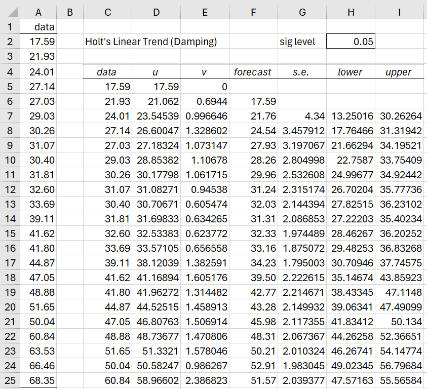
Example 1: Create a forecast for the next 4 years based on the annual data in the range A1:A25 of Figure 2 based on Holt’s Linear Trend with Damping where α = .8, β = .2, and φ = .9.
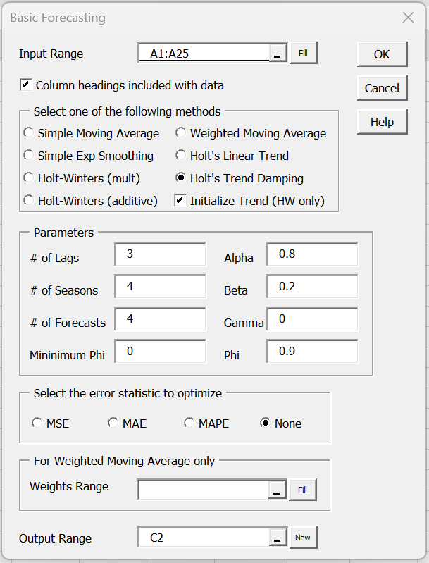
To accomplish this using Real Statistics, press Ctrl-m, and select Basic Forecasting from the Time S tab. Fill in the dialog box that appears as shown in Figure 1, specifying the appropriate values for Alpha, Beta, Phi, and # of Forecasts. Also, make sure that the None optimization option is selected.
Figure 1 – Forecasting Tool dialog box
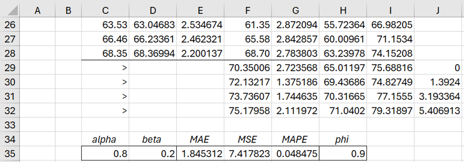
The output is shown in Figures 2, 3, and 4.
Figure 2 – Holt’s Linear Trend with Damping (part 1)
Figure 3 – Holt’s Linear Trend with Damping (part 2)
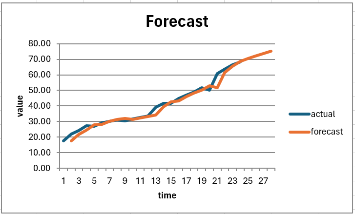
The following figure displays a graph of the forecast.
Figure 4 – Holt’s Linear Trend with Damping (part 3)
We show some representative formulas where the damping version of Holt’s Linear Trend differs from the version without damping in Figure 5.

Figure 5 – Representative Formulas
Optimization Example
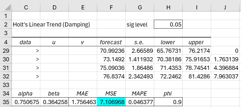
Example 2: Create a forecast for the next 4 years based on the annual data in the range A1:A25 of Figure 2 based on Holt’s Linear Trend with Damping where we optimize alpha and beta based minimizing MSE and with φ = .9.
We again use Real Statistics’ Basic Forecasting tool, as described above, except that this time we use the MSE optimization option. The results are shown in Figure 6 (although rows 5 through 28 are not displayed). Note that the MSE value in Figure 6 is lower than that shown in Figure 3.
Figure 6 – Optimizing Holt’s Linear Trend with damping
Optimizing all three parameters
Note too that the damping parameter in Example 2 is preselected and not optimized. If the Phi field (containing the damping parameter) is set to zero and one of the optimization options (i.e. not None) is chosen then the data analysis tool will optimize the phi parameter as well as the alpha and beta parameters.
Furthermore, you can limit the lower bound on the optimization of phi by inserting a value between 0 and 1 in the Minimum Phi field. For example, if you insert 0 in the Phi field, .8 in the Minimum Phi field, and check MAE optimization, then the data analysis tool will find the alpha, beta, and phi values that minimize MAE restricting phi to a value .8 < φ < 1.
Examples Workbook
Click here to download the Excel workbook with the examples described on this webpage.
References
Gardner, E. S., & McKenzie, E. (1985) Forecasting trends in time series. Management Science, 31(10), 1237–1246.
https://www.bauer.uh.edu/egardner/3301H%20Operations%20Management/ESG%20Publications/1985%20Forecasting%20trends.pdf
Hyndman, R. J., and Athanasopoulos, G. (2018) Holt’s linear trend method. Forecasting: principals and practice, 2nd Ed.
https://otexts.com/fpp2/holt.html


