Key Property
Property 1: For an AR(p) process yi = φ0 + φ1 yi-1 +…+ φp yi-p + εi, PACF(k) = φk
Thus, for k > p, it follows that PACF(k) = 0. See Partial Autocorrelation.
AR(1) Example
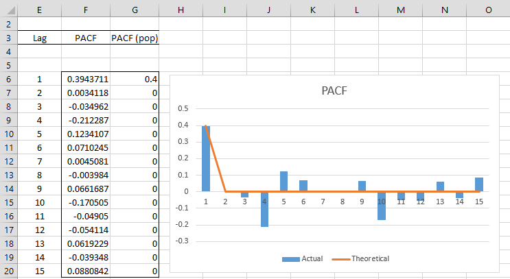
Example 1: Chart PACF for the data in Example 1 from Basic Concepts for Autoregressive Process
Using the PACF function and Property 1, we get the result shown in Figure 1.
Figure 1 – Graph of PACF for AR(1) process
Observation: We see from Figure 1 that the PACF values for lags > 1 are close to zero, as expected, although there is some random fluctuation from zero.
AR(2) Example
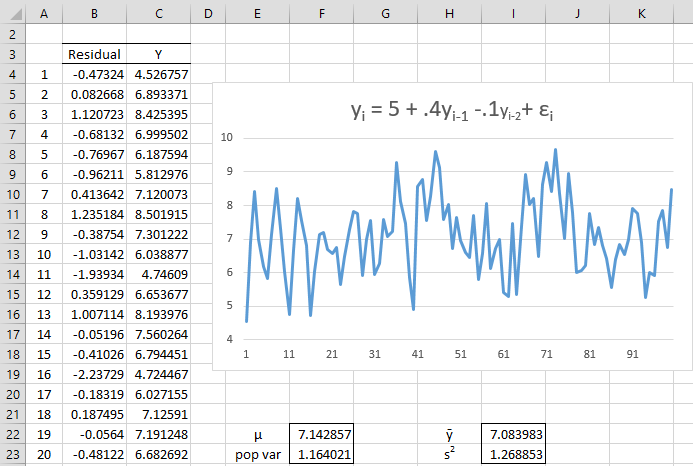
Example 2: Repeat Example 1 for the AR(2) process
where εi ∼ N(0,1), and calculate ACF and PACF.
From Example 2 of Characteristic Equation of AR(p) Process, we know that this process is stationary.
Figure 2 – Simulated AR(2) process
This time, we place the formula =5+0.4*0-0.1*0+B4 in cell C4, =5+0.4*C4-0.1*0+B5 in cell C5, and =5+0.4*C5-0.1*C4+B6 in cell C6, highlight the range C6:C103, and press Ctrl-D.
The ACF and PACF are shown in Figure 3.
Figure 3 – ACF and PACF for AR(2) process
As you can see, there isn’t a perfect fit between the theoretical and actual ACF and PACF values.
Examples Workbook
Click here to download the Excel workbook with the examples described on this webpage.
Links
References
Alonso, A. M., Garcia-Martos, C. (2012) Time series analysis: autoregressive, MA and ARMA processes
https://www.academia.edu/35659911/Time_Series_Analysis_Autoregressive_MA_and_ARMA_processes
Greene, W. H. (2002) Econometric analysis. 5th Ed. Prentice-Hall
https://www.ctanujit.org/uploads/2/5/3/9/25393293/_econometric_analysis_by_greence.pdf
Gujarati, D. & Porter, D. (2009) Basic econometrics. 5th Ed. McGraw Hill
http://www.uop.edu.pk/ocontents/gujarati_book.pdf
Hamilton, J. D. (1994) Time series analysis. Princeton University Press
https://press.princeton.edu/books/hardcover/9780691042893/time-series-analysis
Wooldridge, J. M. (2009) Introductory econometrics, a modern approach. 5th Ed. South-Western, Cegage Learning
https://cbpbu.ac.in/userfiles/file/2020/STUDY_MAT/ECO/2.pdf


how to decide the upper limit and Lower Limit of ACF? is it always 0.2?
Hello Adam,
I don’t know what you are referring to. Where did you get the .2 value? Please explain in more detail.
Charles
+-2/sqrt(n)
Adam,
I don’t see lower and upper bounds on this webpage, nor do I see any reference to .2 or 2/sqrtn). Are you referencing a different webpage?
Charles