Real Statistics ARMA Tool

We now show how to create an ARMA model of a time series using the ARIMA Real Statistics data analysis tool and to use this model to create a forecast.

The data analysis tool uses the Real Statistics ARIMA_Coeff function (described in detail below) to calculate the ARMA coefficients along with their standard errors. This function uses the Levenberg-Marquardt algorithm instead of Solver, resulting in a more accurate model (i.e. one with a lower SSE value).

Real Statistics Data Analysis Tool: The Real Statistics Resource Pack provides the ARIMA Model and Forecast data analysis tool which tries to fit an ARMA(p, q) process to time series data. This tool can also be used to analyze an ARIMA process as demonstrated in ARIMA Model Coefficients.

Example 1: Use the ARIMA Model and Forecast data analysis tool to build an ARMA(2,1) model for the data in Example 2 of Calculating ARMA Coefficients using Solver (the first 20 elements in the time series are repeated in Figure 1).

Start by pressing Ctr-m and choosing the Time Series option. Select the ARIMA Model and Forecast option on the dialog box that appears and click on the OK button. Now, fill in the dialog box that appears as shown in Figure 1.

Figure 1 – ARIMA Model and Forecast dialog box

In Figure 1 we have inserted the time series values in the Input Range field, without column heading or sequence numbers. We also insert the p value in the AR order field and the q value in the MA order field. We also check the Constant included in the model field. Since we want to forecast 5 additional elements, we insert 5 in the # of Forecasts field. We will describe the other options later.

When we click on the OK button, we see the output shown in Figures 2, 3 and 4.

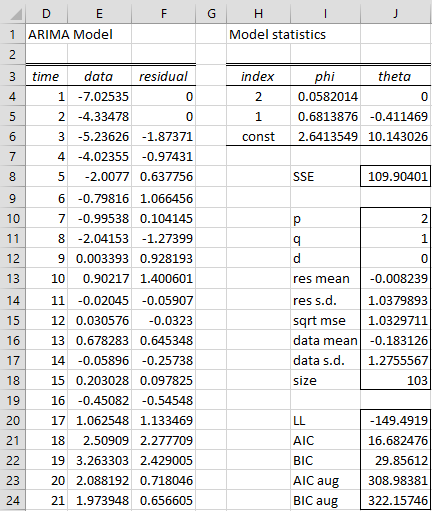
Figure 2 – ARMA(2,1) model – part 1

In Figure 2, we see that the best fit ARMA(2,1) process is given by

y_i = 2.64 + .68y_i-1 + .06y_i-2 + ε_i – .41ε_i-1

The mean value 10.143026 (cell J6) has been subtracted from all the y values in column B (shown in Figure 1) to obtain the z values in column E.

Note that the formula in cell F6 is

=E6-SUMPRODUCT(E4:E5,I$4:I$5)-SUMPRODUCT(F4:F5,J$4:J$5)

Similar formulas are used to calculate the other residual values shown in column F. The formula used to calculate SSE (cell J8) is =SUMSQ(F6:F108). The other cells are calculated as described in Evaluating the ARMA Model.

Note that AIC = 16.68 (cell J21). This compares with AIC = 13.03 for the ARMA(1,1) model used to fit the same data as shown in Figure 2 of Evaluating the ARMA Model. This gives evidence that the ARMA(1,1) model is a better fit for the data than the ARMA(2,1) model. Similarly, BIC = 29.86 (cell J22) for the ARMA(2,1) model is greater than BIC = 20.30 for the ARMA(1,1) model shown in Figure 2 of Evaluating the ARMA Model, giving more evidence that the ARMA(1,1) is the better, and certainly more parsimonious, fit for the data.

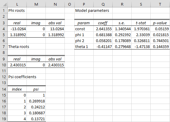
Figure 3 – ARMA(2,1) model – part 2

From Figure 3, we see that the ARMA(2,1) process is both stationary and invertible (since the absolute values of all the roots are greater than 1).

The coefficient values and their standard errors are calculated by the Real Statistics array formula =ARIMA_Coeff(B4:B108,2,1,0,TRUE) in range Q4:R7. Cell S4 contains the formula =Q4/R4 and cell S5 contains the formula =T.DIST.2T(ABS(S4),J$18-J$10-J$11-1). The output in range P3:T7 uses a different approach from that employed in Figure 3 are given in Evaluating the ARMA Model.

We see that only the constant and phi 1 coefficients are making a significant contribution to the LL value of the ARMA(2,1) model (since these are the only ones whose p-value < .05 = α).

The psi coefficients in range M16:M20 are used to create the forecast values and are calculated using the array formula =PSICoeff(I4:I5,J4:J5). Five psi coefficient values are produced since we requested 5 forecast values.

More details about the values in Figure 3 are given in Evaluating the ARMA Model.

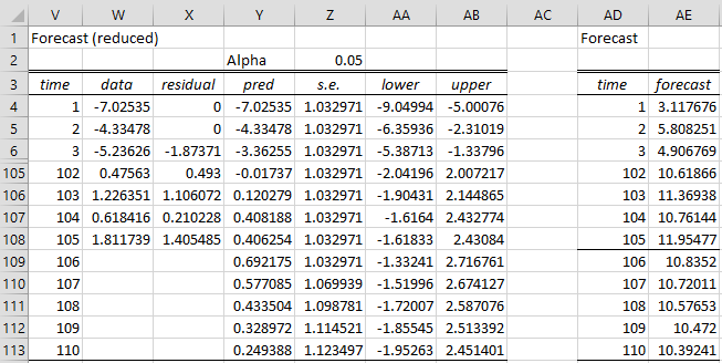
Finally, we show the forecast values in Figure 4.

Figure 4 – ARMA(2,1) model – part 3

To save space, we have not included the values for times 4 through 101. Note the following formulas used in Figure 4.

Cell	Entry	Formula
X109	pred z106	=SUMPRODUCT(V107:V108,I$4:I$5)+SUMPRODUCT(W107:W108,J$4:J$5)
X110	pred z107	=SUMPRODUCT(V108,I4)+SUMPRODUCT(X109,I5)+SUMPRODUCT(W108,J4)
X111	pred z108	=SUMPRODUCT(X109:X110,I4:I5)
X112	pred z109	=SUMPRODUCT(X110:X111,I4:I5)
X113	pred z110	=SUMPRODUCT(X111:X112,I4:I5)
Y113	s.e.	=J$15*SQRT(SUMSQ(M$16:M20))
AD113	pred y110	=X113+J$6

Figure 5 – Formulas from Figure 4

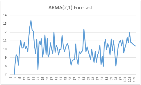
We show the time series plus 5 forecasted elements in Figure 6 based on the data in range AD4:AD113 of Figure 4.

Figure 6 – Time series forecast

See ARMA Tool Options for a description of the following options that are displayed in Figure 1:

• Make AR(p) agree with OLS
• Include sigma-sq in AIC/BIC
• Reformat for Linear Regression
• Use Solver

Real Statistics Function: The Real Statistics Resource Pack provides the following array functions. In particular, the first function is used to calculate the ARIMA coefficients and their standard errors.

ARIMA_Coeff(R1, p, q, d, con, lab) = a p+q+1 × 4 array, each row of which contains the coefficient, standard error, t-stat and p-value (in order: constant, phi 1, phi 2, …, theta 1, theta 2, …) of the ARIMA(p,q,d) model for the time series data in column range R1; if lab = TRUE (default FALSE), then an extra row and column are appended with labels; if con = TRUE (default) then a constant term is used, otherwise it is not (i.e. it is set to zero).

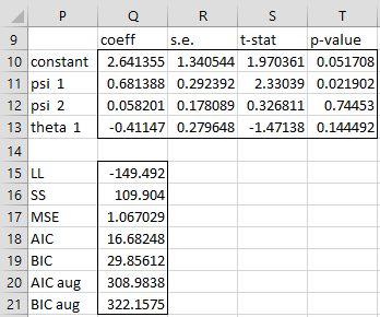
Range Q4:R7 of Figure 3 contains the formula =ARIMA_Coeff(B4:B108,2,1,0,TRUE), where only the first two columns of the output are used (with no labels). The output from the array formula =ARIMA_Coeff(B4:B108,2,1,0,TRUE,TRUE) is shown in range P9:T13 of Figure 7.

Figure 7 – ARIMA_Coeff and ARIMA_Stats functions

Note too that there are more options for the con argument than just TRUE and FALSE. In fact, you can specify a column or row range with up to p+q+1 elements. Each position in the range specifies the initial guess used for the corresponding coefficient in the Levenberg-Marquardt algorithm. The initial guess for any coefficients that are not explicitly specified is .2. Note too that if the element in the range takes the form “c” followed by a numeric value, then that numeric value will be fixed and the Levenberg-Marquardt algorithm will not change it.

E.g. for an ARIMA(2,1,0) model, the con range can have up to p+q+1 = 2+1+1 = 4 elements, the first for the constant, the second for phi 1, the third for phi 2 and the fourth for theta 1. Thus, if cell D1 contains “c1.2” and cell D2 contains .4, then the formula =ARIMA_Coeff(B4:B108,2,1,0,D1:D2) specifies that the constant term will be fixed with the value 1.2 and phi 1 will be initialized to .4 (instead of .2) although its final value will depend on the Levenberg-Marquardt algorithm. The initial values of phi 2 and theta 1 will be .2 (the default) since these values have not been specified in range D1:D2.

ARIMA_Stats(R1,R2, p, q, d, con, lab) = 7 × 1 column array containing the values LL, SSE, MSE, AIC, BIC, AIC augmented and BIC augmented for the ARIMA(p,q,d) model for the time series data in column range R1 based on the coefficients in the p+q+1 × 1 column range R2; if lab = TRUE (default FALSE), then an extra column of labels is appended to the output; if con = TRUE (default) then a constant term is used, otherwise it is not (unlike ARIMA_Coeff, no other values are acceptable).

The output from the array formula =ARIMA_Stats(B4:B108,Q10:Q13,2,1,0,,TRUE) is shown in range P15:Q21 of Figure 7.

References

Pelgrin, F. (2011) Estimation of ARIMA models
https://math.univ-cotedazur.fr/~frapetti/CorsoP/Chapitre_4_IMEA_1.pdf
Triacca, U. (2014) Estimation of the parameters of an ARMA model
No longer available online
Hamilton, J. D. (1994) Time series analysis. Princeton University Press
https://press.princeton.edu/books/hardcover/9780691042893/time-series-analysis
Hitchcock, D. (2016) Parameter estimation in time series models
https://people.stat.sc.edu/Hitchcock/stat520ch7slides.pdf
Wikipedia (2016) Levenberg-Marquardt algorithm
https://en.wikipedia.org/wiki/Levenberg%E2%80%93Marquardt_algorithm
Hi Charles,
Hope you are well.
You mentioned that one of your functions use the Levenberg-Marquardt algorithm. Is there any appetite to unpack this algorithm? I’ve just started looking at it and I can see it’s no easy feat with Jacobian matrices etc.
kind regards
Declan
Hi Declan,
This is on my list of future enhancements.
Charles
Figure 1, what are the values of B24:B108?
Hello Dean,
You can download all the spreadsheets used on the website via the following link:
https://www.real-statistics.com/free-download/real-statistics-examples-workbook/
You need to download the Time Series Analysis examples workbook.
Dear Charles,
Thank you for the extensive and good info that we can find in your site!
I was trying to run ARIMA in a similar fashion to the example above using the Real Statistics add in and I am getting this message when I press ” OK” in the ARIMA model dialog box:
” Compile error in hidden module: ‘TimeSeries’. This error commonly occurs when code is incompatible with the version, platform, or architecture of this application.”
I run Excel 365 version 16.27 on a Mac running macOS Mojave 10.14.5.
Would you be able to help with this?
Thanks a lot,
Andre
Hello Andre,
When you select Add-Ins from the Tools menu, do you see RealStats-Mac-2016 and Solver on the list of add-ins with check marks next to them? What do you see when you enter the formula =VER() into any cell?
Hello Charles,
Thanks for the quick reply!
Selecting “Tools” and “Excel Add-ins” I see both RealStats-Mac-2016 and Solver on the list of add-ins with check marks next to them. I have used Solver extensively in the past so this is running Ok and I am using the functions on the RealStats add-in as well, the only issue so far is when I was running “Time Series” / “ARIMA”.
Entering the formula =VER() I get: 6.4 Excel 2016/2019/365 Mac
Thanks for your support.
André
If you email an Excel file with your data I will try to figure out what is going wrong.
Thanks again for the help with the previous error. Now I have calculated ARIMA for a time series that I have and using different configurations I arrived in the following AIC and BIC values, all negative and rounded for convenience:
ARIMA(2,1,1) with phi0: AIC = -29 & BIC=-20
ARIMA(2,1,1) w/o phi0: AIC = -21 & BIC=-13
ARIMA(1,1,1) w/o phi0: AIC = -16 & BIC=-10
My interpretation is that ARIMA(1,1,1) fits better. Is that correct? Thanks again!
Based on the AIC and BIC values, ARIMA(2,1,1) with constant seems to be the best of the three choices (lowest AIC and BIC values).
I have time series data and the data show 3 distinct trends, How can apply a standard method to identify the trends.
Thank you
AM
Hello Ahmed,
This depends on the details. If each trend applies to different time periods, perhaps you can split the data into three time series.
When I try using the ARIMA model, I get the following message:
“Run-time error 438:
Object does not support this property or method”.
What does this mean and what do I need to do to fix this?
Thanks
Sumi,
It probably means that Solver is not installed on your version of Excel. When you press Alt-TI do you see Solver on the list of addins with a check mark next to it?
Thanks for sharing the knowledge about ARIMA.
Charles, I have the question for you. I want to predict the number of cases. As example, I used weekly data. The data range from Week 1 to Week 10 for year 2010. Then i fill in the prediction number is 10. Is it the result shows the forecasting cases for;
1) Week 11 to Week 20 for year 2010; OR
2) Week 1 to Week 10 for year 2011?
I really appreciate if you can help me. Thanks a lot Charles.
Ei,
The result should be the next 10 weeks after the data in the input range, which in your case should be week 11 to 20 for the year 2010 (i.e. option 1).
Hi Charles
I am attempting to run ARIMA model. When I click ok I get this error; “Compile error in hidden module: ‘TimeSeries’. This error commonly occurs when code is incompatible with the version, platform, or architecture of this application.”
Other functions are working fine so far (including those in the time series menu), the ARIMA model is the first I’ve had an issue with.
Chris,
The usual reason for this error message is that Solver is not activated. You can check this by pressing Alt-TI and seeing whether Solver appears in the list of addins with a check mark next to it.
Since the other data analysis tools are working, this may not be the problem in your case. If you send me an Excel file with your data and clear instructions as to what values you used in the ARIMA dialog box, I will try to figure out what is the source of this error.
Also you should look at the Troubleshooting section of this webpage.
Thanks Charles for the response. I look forward to the update.
Is there a way to integrate ARMA with a standard regression model i.e. run a regression with an AR (or ARMAX) term applied to the error term of a regression model suffering from serial correlation?
For example say I have run an OLS regression with 5 independent variable but when I test the residuals from the model they suffer from high level of autocorrelation invalidating the accuracy of the coefficients/Standard errors. I would like to re-estimate the model including an ar term for the residuals error term to eliminate the serial correlation and thereby re-estimate the coefficients.
Joel
Joel,
Yes, there are ways to perform regression which takes autocorrelation into account. Typical approaches use GLS instead of OLS and Newey-West method.
I am planning to add this topic to the website and software shortly.