Forecasting using an ARMA model

We now show how to create forecasts for a time series modelled by an ARMA(p,q) process.

Example 1: Create a forecast for times 106 through 110 based on the ARMA(1,1) model created in Example 1 of Calculating ARMA Coefficients using Solver.

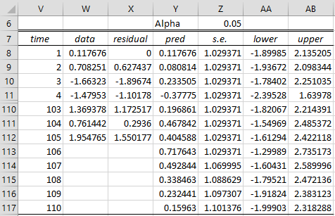
The result is shown in Figure 1, where we have omitted the data for times 5 through 102 to save space.

Figure 1 – Forecast for AR(1,1) process

Columns V, W and X are just copies of columns E, F and G from Figure 1 of Calculating ARMA Coefficients using Solver. The predicted values in Y for the observed data in the time series (range Y8:Y112) is simply the data element minus the residual; e.g. cell Y8 contains the formula =W8-X8.

The predicted (or forecasted) value at time 106 (cell Y113) is based on the equation that defines the ARIMA(1,1) process, namely

Thus, the forecast value at time i = 106 is

Note that since we don’t have an observed value for ε₁₀₆, we use the theoretical mean value, namely zero. The forecasted value at time i = 106 is calculated in Figure 1 using the formula =SUMPRODUCT(W112,J$8)+SUMPRODUCT(X112,K$8). For this model, this formula can be simplified to =W112*J8+X112*K8, but the longer formula will come in handy when we create forecasts using ARMA(p, q) where p and/or q is larger than 1.

The forecast at time i = 107 is calculated by

This time, there are no observed values for ε₁₀₆, ε₁₀₇, or y₁₀₆. As before, we estimate ε₁₀₆ and ε₁₀₇ by zero, but we estimate y₁₀₆ by the forecasted value ŷ₁₀₆. This is accomplished in Excel using the formula =SUMPRODUCT(Y113,J8).

The forecasted values at times 108, 109 and 110 are calculated in a similar manner.

We next look at the standard error for the forecast values. For the observed times, the standard error is σ, which can be estimated by  = =  = 1.029371, where SSE = 110.19884 (see Figure 2 of Calculating ARMA Coefficients using Solver).

The standard error of the m^th forecasted value (after the n observed values) is given by the formula

where

is the MA(∞) representation of the ARMA process. As before, we estimate σ by estimated by = 1.029371.

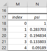
The psi coefficients for the MA(∞) representation are as shown in Figure 2.

Figure 2 – Psi coefficients for MA(∞) representation

Here the formula =PSICoeff(J8,K8) is inserted in range N18:N22.

Thus, for example, the standard error for ŷ₁₀₈ is

This value is calculated (cell Z115) by the formula =K$18*SQRT(SUMSQ(N$18:N20)).

The 95% confidence interval for ŷ₁₀₈ is therefore

which is (-1.79521, 2.472136), as shown on row 115 of Figure 1. For example, the formula in cell AB115 is =Y115+NORMSINV(1-Z$6/2)*Z115.

Example 2: Create a forecast for times 106 through 110 based on the ARMA(1,1) model created in Example 2 of Calculating ARMA Coefficients using Solver.

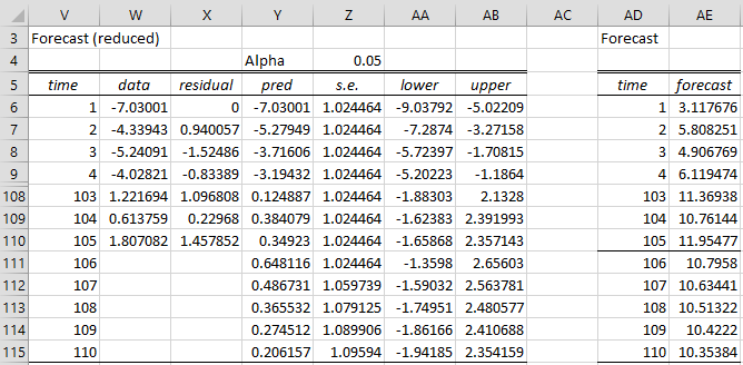
The process is identical to that shown in Example 1. The only difference is that this time there is a constant term in the ARMA(1,1) model. The result is shown in Figure 3.

Figure 3 – Forecast for ARMA(1,1) process with non-zero mean

As we discussed in Evaluating the ARMA Model, the left side of Figure 3 contains the forecast not for the original y_i data, but for the z_i data where z_i = y_i – µ, where the estimate for µ is 10.147687 (cell K7 in Figure 4 of Calculating ARMA Coefficients using Solver). To create a forecast for the y_i time series, we need to add 10.147687 to the forecasted z_i values. This is done in column AE,

E.g., cell AE115 contains the formula =Y115+K7, while cell AE6 contains the formula =W6+K7.

References

Triacca, U. (2014) Forecasting stationary time series
https:// No longer available online
Hamilton, J. D. (1994) Time series analysis. Princeton University Press
https://press.princeton.edu/books/hardcover/9780691042893/time-series-analysis
Hitchcock, D. (2016) Forecasting
https://people.stat.sc.edu/hitchcock/stat520ch9slides.pdf