ARMA(1,1) Processes

MA(∞) Representation

For an ARMA(1, 1) process

Now let’s suppose that |φ₁| < 1. We show how to create the MA(∞) representation as follows:

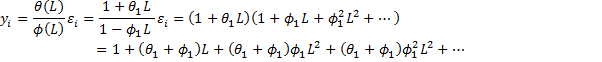
Thus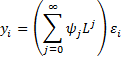

where ψ₀ = 1 and for j > 0

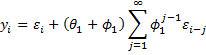
The MA(∞) representation is therefore

If |φ₁| < 1, then this ARMA(1,1) process is stationary. It also turns out that when |θ₁| < 1, the process is invertible.

Example 1: Find the MA(∞) form of the ARMA(1, 1) process y_i =.4y_i-1 +ε_i – .2ε_i-1

etc.

We get the same result using the Real Statistics PSICoeff array function as shown in Figure 1.

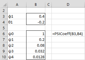
Figure 1 – Finding MA(∞) Coefficients

Properties

Property 1: The following is true for an ARMA(1, 1) process

Proof: See ARMA Proofs

Property 2: The following is true for an ARMA(1, 1) process

and for k > 1

Proof: See ARMA Proofs

Observation: Since z₁ = 1/φ₁ is the root of the characteristic polynomial φ(z) = 1 – φ₁z, we can express the second term in Property 2 as

It turns out that this can be generalized to other ARMA processes.

Property 3: The following is true for an ARMA(1, 1) process

and for k > 1

Proof: See ARMA Proofs

Estimating Coefficients

As we discuss elsewhere, we can use MLE or Solver to estimate the coefficients of an ARMA(1, 1) process. Here we show how to use the ACF to estimate these coefficients.

Given a time series from an ARMA(1, 1) process, we can calculate r₁ and r₂ as estimates of ρ₁ and ρ₂. Now by Property 3, ρ₂ = ρ₁φ₁, and so φ₁ = ρ₂/ρ₁. We can now plug these values into the other formula from Property 3

to obtain an estimate for θ₁. In fact, we can express this formula as

Using the quadratic formula, we keep any real invertible solution for θ₁, if it exists. We can calculate the variance of the error via the formula

where s² is the usual expression for the variance of the time series

Restriction

When θ₁ = –φ₁ for an ARMA(1, 1) process, we note that γ₀ = σ² and ρ_k = 0 for all k > 1, which are the characteristics of white noise.

In fact, the white noise process with zero mean takes the form

y_i = ε_i

We see that φ₁ y_i – φ₁ ε_i  = 0  for all i, and in particular φ₁ y_i-1 – φ₁ ε_i-1  = 0. Thus, the process takes the form

which is an ARMA(1,1) process with θ₁ = –φ₁. In fact, when this ARMA process is expressed in lag format as

φ(L)y_i = θ(L)ε_i

then φ(L) and θ(L) have a common factor, namely 1 – φ₁. Henceforth we insist that an ARMA model not have a common factor, and so the above model can’t be expressed as an ARMA(1,1) model.

Simulation (zero mean)

Example 2: Simulate a sample of 105 elements from the ARMA(1, 1) process

where ε_i ∼ N(0, 1) and calculate the ACF.

This is done in Figure 2 by placing the formula =NORM.S.INV(RAND()) in cell B7 and the formula =0.7*C6+B7-0.2*B6 in cell C7, highlighting the range B7:C111 and pressing Ctrl-D (only the first 16 elements of the simulation is shown in Figure 2).

Figure 2 – Simulated ARMA(1,1) process

The ACF values are shown in Figure 3 where the theoretical values are based on Property 3.

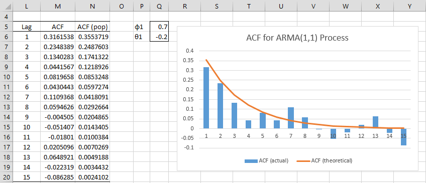
Figure 3 – ACF for ARMA(1,1) Process

Cell M6 contains the formula =ACF($C$12:$C$111,L6), and similarly, for the other cells in column M, cell N6 contains the formula =(Q5+Q6)*(1+Q5*Q6)/(1+2*Q5*Q6+Q5^2) and cell N7 contains the formula =N6*Q$5, and similarly for rest of the cells in column N.

Since |φ₁| = .7 < 1 and |θ₁| = .2 < 1, this process is both stationary and invertible.

Simulation (non-zero mean)

Example 3: Simulate a sample of 105 elements from the ARMA(1, 1) process

where ε_i ∼ N(0, 1) and calculate the ACF.

The only difference between this process and the one in Example 2 is the constant term. The approach is identical, except that this time you place the formula =3+0.7*C6+B7-0.2*B6 in cell C7. The result is shown in Figure 4. Note that the ACF values are identical to those in Figure 3.

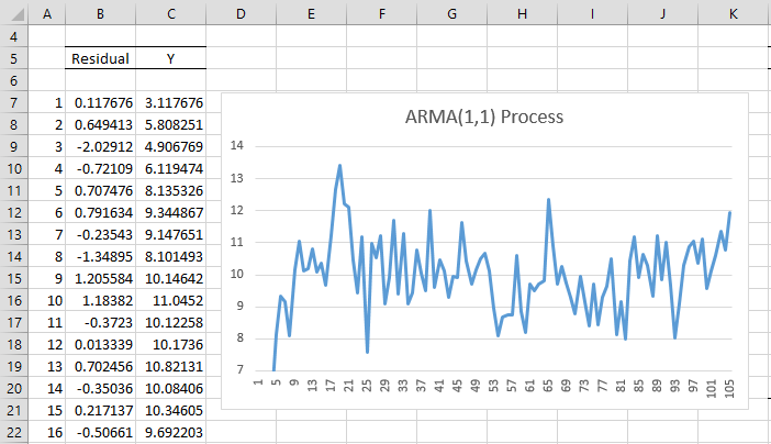
Figure 4 – Simulated ARMA(1,1) Process with non-zero mean

Examples Workbook

Click here to download the Excel workbook with the examples described on this webpage.

References

Greene, W. H. (2002) Econometric analysis. 5th Ed. Prentice-Hall
https://www.scirp.org/(S(351jmbntvnsjt1aadkposzje))/reference/referencespapers.aspx?referenceid=1243286

Gujarati, D. & Porter, D. (2009) Basic econometrics. 5th Ed. McGraw Hill
http://www.uop.edu.pk/ocontents/gujarati_book.pdf

Hamilton, J. D. (1994) Time series analysis. Princeton University Press
https://press.princeton.edu/books/hardcover/9780691042893/time-series-analysis

Wooldridge, J. M. (2009) Introductory econometrics, a modern approach. 5th Ed. South-Western, Cegage Learning
https://cbpbu.ac.in/userfiles/file/2020/STUDY_MAT/ECO/2.pdf

Wei, W. (2006) Time series analysis: univariate and multivariate methods, 2nd edition. Pearson Addison Wesley https://www.researchgate.net/publication/236651810_Time_Series_Analysis_Univariate_and_Multivariate_Methods_2nd_edition_2006