Assumptions
The t distribution provides a good way to perform one-sample tests on the mean when the population variance is not known provided the population is normal or the sample is sufficiently large so that the Central Limit Theorem applies (see Properties 1 and 2 of Basic Concepts of t Distribution).
It turns out that the one-sample t-test is quite robust to moderate violations of normality. In particular, the test provides good results even when the population is not normal or the sample size is small, provided that the sample is reasonably symmetrically distributed about the sample mean. This can be determined by graphing the data. The following are indications of symmetry:
- The boxplot is relatively symmetrical; i.e. the median is in the center of the box and the whiskers extend equally in each direction
- The histogram looks symmetrical
- The mean is approximately equal to the median
- The coefficient of skewness is relatively small
The impact of non-normality is less for a two-tailed test than for a one-tailed test and for higher alpha values than for lower alpha values.
The other assumption for the t-test is that we have a random sample. If, for example, we are interested in the mean cholesterol level of a population, then our sample must consist of the cholesterol levels of people chosen at random. We can’t use the t-test for a sample consisting of cholesterol levels for the same person at different points in time.
One-tailed t-test
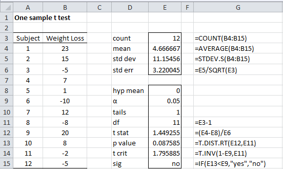
Example 1: A weight reduction program claims to be effective in treating obesity. To test this claim 12 people were put on the program and the number of pounds of weight gain/loss was recorded for each person after two years, as shown in columns A and B of Figure 1. Can we conclude that the program is effective?
Figure 1 – One sample t-test
A negative value in column B indicates that the subject gained weight. We judge the program to be effective if there is some weight loss at the 95% significance level. Usually, we conduct a two-tailed test since there is a risk that the program might actually result in weight gain rather than loss, but for this example, we will conduct a one-tailed test (perhaps because we have evidence, e.g. from an earlier study, that overall weight gain is unlikely). Thus our null hypothesis is:
H0: μ ≤ 0; i.e. the program is not effective
Testing Assumptions
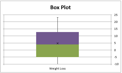
From the box plot in Figure 2, we see that the data is quite symmetric and so we use the t-test even though the sample is small.
Figure 2 – Box plot for sample data
Test Results
Column E of Figure 1 contains all the formulas required to carry out the t-test. Since Excel only displays the values of these formulas, we show each of the formulas (in text format) in column G so that you can see how the calculations are performed.
We see that n = 12, x̄ = 4.67, s = 11.15 and s.e. = s ⁄ = 3.22. We now conclude that
with df = 11 degrees of freedom.
Since p-value = T.DIST.RT(t, df) = T.DIST.RT(1.45, 11) = .088 > .05 = α, the null hypothesis is not rejected. This means there is an 8.8% probability of achieving a value for t this high assuming that the null hypothesis is true, and since 8.8% > 5% we can’t reject the null hypothesis.
The same conclusion is reached since
tcrit = T.INV(1-α, df) = T.INV(.95, 11) = 1.80 > 1.45 = tobs
Note that if we had used the normal distribution for the hypothesis testing as described in Sampling Distributions we would have gotten the following result:
NORM.DIST(x, μ, σ, TRUE) = NORM.DIST(4.67, 0, 11.15, TRUE) = .926 < .95 = 1 – α
This would again show that the null hypothesis can’t be rejected. We see that the probability of being in the critical range is .074 compared to .088 in the t-distribution case. In fact, the large sample test (via the normal distribution) is not as accurate as the small sample t-test.
Two-tailed t-test
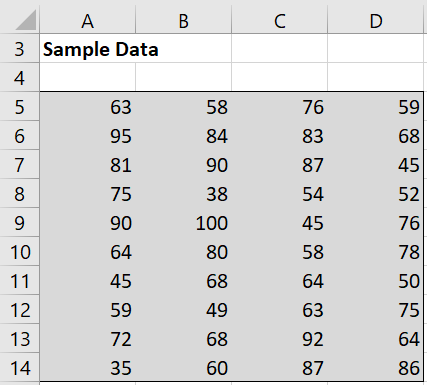
Example 2: A school board wanted to see if reading test scores have changed in the past 30 years by testing a random sample of 40 students to see whether there is a significant change from the average score of 78 thirty years ago. The scores in the sample are shown in Figure 3.
Figure 3 – Random sample data
Based on this data, can we claim that the reading scores have changed in the past 30 years?
We will test the two-sided null hypothesis:
H0: µ = 78
Normality Assumption
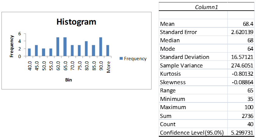
From Excel’s Histogram data analysis tool, we see that the data is reasonably symmetric. This is confirmed by Excel’s Descriptive Statistics data analysis tool since the mean and median are approximately equal and the skewness is close to zero (see Figure 4). This justifies the use of a t-test.
Figure 4 – Testing for symmetry
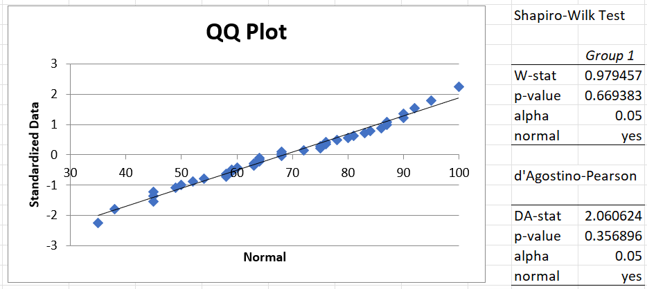
Actually, we can use the QQ-Plot and Shapiro-Wilk options of the Real Statistics Descriptive Statistics and Normality data analysis tool, as shown in Figure 5, to demonstrate directly that the data satisfy the normality assumption.
Figure 5 – Testing for normality
Data Analysis Tool
This time we will use a Real Statistics data analysis tool to perform the analysis.
Real Statistics Data Analysis Tool: The Real Statistics Resource Pack provides a data analysis tool called T Tests and Non-parametric Equivalents, which provides access to the t-test for one sample, two independent samples, and paired samples, as well as the non-parametric equivalent tests (Mann-Whitney and Wilcoxon Signed-Ranks tests).
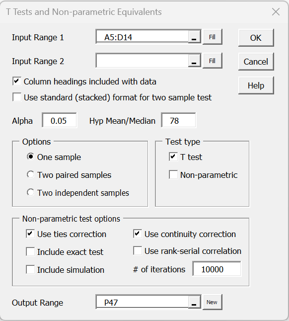
For Example 2, enter Ctrl-m and select T Tests and Non-parametric Equivalents from the menu (or from the Misc tab when using the Multipage interface). A dialog box will appear as displayed in Figure 6.
Figure 6 – Dialog box for T Tests and Non-parametric Equivalents
Enter A5:D14 in the Input Range and 78 for the Hypothetical Mean/Median, unclick Column headings included with data, and choose the One sample and T test options. When you click on the OK button, the output shown in Figure 7 is displayed.
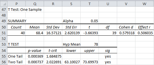
Figure 7 – Real Statistics one-sample t-test
Analysis
From the figure, we see that
with n – 1 = 39 degrees of freedom.
Thus, p-value = T.DIST.2T(ABS(t), df) = T.DIST.2T(3.66, 39) = .00074 < .05 = α, and so we reject the null hypothesis and conclude there is a significant change (i.e. reduction) in the test scores.
Alternatively we can calculate, tcrit = T.INV.2T(α, df) = T.INV.2T(.05, 39) = 2.02. Since |tobs| = 3.66 > 2.02 once again we reject the null hypothesis.
Note that in Excel 2007 we calculate p-value = TDIST(t, df, 2) = TDIST(3.66, 39, 2) = .00074 < .05 = α.
The input data for the one-sample t-test can have missing data, indicated by empty cells or cells with non-numeric data. Such cells will be ignored in the analysis.
Worksheet Function
As described in Paired T-Test and Two-Sample T-Test, Excel provides a T.TEST function that supports paired-sample and two-sample t-tests, but not the one-sample t-test. The following Real Statistics function fills in this gap.
Real Statistics Function: The Real Statistics Resource Pack provides the following function:
T1_TEST (R1, hyp, tails) = the p-value of the one-sample t-test for the data in array R1 based on the hypothetical mean hyp (default 0) where tails = 1 or 2 (default).
For Example 2, the formula T1_TEST(A5:D14, 78, 2) will output the same value shown in cell Q56 of Figure 5, namely p-value = .000737.
Confidence interval
As described in Confidence Intervals for Sampling Distributions, we can define the confidence interval associated with the t distribution as
observed mean ± tcrit ⋅ std error
Example 3: Calculate the 95% confidence interval for Example 2
meanobs ± tcrit ⋅ std err = 68.40 ± 2.02 ⋅ 2.62 = 68.40 ± 5.30
This yields a 95% confidence interval of (63.10, 73.70). Since the interval doesn’t contain the hypothetical mean of 78, once again we are justified in rejecting the null hypothesis (with 95% confidence).
Note that the endpoints of the confidence interval, 63.10 and 73.70, are displayed in cells S56 and T56 of Figure 7.
Excel Function
Versions of Excel starting with Excel 2010 provide the following function to calculate the confidence interval for the t distribution.
CONFIDENCE.T(α, s, n) = k such that (x̄ – k, x̄ + k) is the confidence interval of the sample mean; i.e. CONFIDENCE.T(α, s, n) = tcrit ∙ std error, where n = sample size, s = sample standard deviation and 100(1 – α) is the confidence percentage.
For Example 2, CONFIDENCE.T(.05,16.57,40) = 5.30 which yields a 95% confidence interval of (68.40 – 5.30, 68.40 + 5.30) = (63.10, 73.70). The same result was obtained from the T Test and Non-parametric Equivalents data analysis tool, as shown in range D56:T56 of Figure 5.
Observation
Excel’s Descriptive Statistics data analysis tool has an option for generating the confidence interval for a sample or collection of samples using the t distribution. Referring to Figure 2 of Descriptive Statistics Tools, to choose this option click on the Confidence Interval for Mean checkbox and specify the confidence percentage (i.e. 1 – α) if you want to override the default of 95%. E.g. from Figure 4, we see that the 95% confidence interval value in the Descriptive Statistics output for the data in Example 2 is 5.299731.
Real Statistics Functions
The Real Statistics Resource Pack provides the following functions:
STDERR(R1) = standard error of the data in the range R1 = STDEV(R1) / SQRT(COUNT(R1))
CONFIDENCE_T(α, s, n) – equivalent to CONFIDENCE.T(α, s, n); useful for Excel 2007 and earlier versions of Excel
T_CONF(R1, α) = k such that (x̄ – k, x̄ + k) is the 1 – α confidence interval of the sample mean for the data in range R1 based on the t distribution
T_LOWER(R1, α) = the lower end, x̄ – k, of the 1 – α confidence interval of the sample mean for the data in range R1 based on the t distribution
T_UPPER(R1, α) = the upper end, x̄ + k, of the 1 – α confidence interval of the sample mean for the data in range R1 based on the t distribution
If α is omitted it defaults to .05. These functions ignore any empty or non-numeric cells.
One-tailed Confidence Interval
Example 4: Calculate the one-tailed 95% confidence interval for Example 1.
Since the null hypothesis is H0: μ ≤ 0, the one-tailed confidence interval for the population mean takes the form
(x̄ – s.e. ⋅ tcrit, ∞)
where tcrit is the one-tailed critical value From Figure 1, we see that
x̄ – s.e. ⋅ tcrit = 4.66667 – 3.220048 ⋅ 1.795885 = -1.110616
Since 0 lies in the confidence interval (-1.11616, ∞), we again conclude that there isn’t sufficient evidence to reject the null hypothesis.
Note that if the null hypothesis were H0: μ ≥ 0, then the one-tailed confidence interval would be
(-∞, x̄ + s.e. ⋅ tcrit)
Prediction interval
Suppose that the mean and standard deviation of a random sample of size n are x̄ and s, respectively. We can then estimate the mean of a new sample of size m to also be x̄. The precision of this prediction would then be
This is called the 1 – α prediction interval.
Example 5: Calculate the 95% prediction interval of one additional data element randomly selected from the population from Example 2.
From Figure 7, we see that x̄ = 68.40, s2 = 274.6051, n = 40, and tcrit = 2.0227 (two-tailed with α = .05). Thus the 95% prediction interval for one additional data element is
and so the prediction interval is (34.47, 102.33). Note that the prediction interval for the mean of another random sample with 40 elements would be (60.91, 75.89), which would be a narrower interval. In any case, this is wider than the 95% confidence interval of (63.10, 73.70). In fact, it is easy to see that the prediction interval is always larger than the confidence interval.
Effect size
Click here for a description of Cohen’s d and Hedges’s g effect size measures for the one-sample t-test. In addition, an estimate of the confidence interval for Cohen’s d is provided.
Statistical Power and Sample Size
Click here for a description of how to calculate the power of a t-test using the same approach as we did in Power of a Sample for the normal distribution. We also show how to estimate the minimum sample size required for a one-sample t-test.
In Statistical Power of the t Tests we show another way of computing statistical power using the noncentral t distribution.
Examples Workbook
Click here to download the Excel workbook with the examples described on this webpage.
References
Howell, D. C. (2010) Statistical methods for psychology (7th ed.). Wadsworth, Cengage Learning.
https://labs.la.utexas.edu/gilden/files/2016/05/Statistics-Text.pdf
Nelson, S. L. and Nelson, E. C. (2016) How to use the t-test data analysis tool in Excel
https://www.dummies.com/article/technology/software/microsoft-products/excel/how-to-use-the-t-test-data-analysis-tool-in-excel-152093/
Zar. J. H. (2010) Biostatistical analysis 5th Ed. Pearson


Dr. Zaiontz,
First thanks for your work on Real Statistics. I use this extensively, and it is extremely useful!
One small comment though; it would seem that your T1_Test function returns negative p-values. The absolute value is correct, but the negative sign is a bit offputting?
Thanks
Hello Jacques,
Can you give me an example of a negative p-value? Keep in mind that when Excel uses scientific notation a value such as -1.0E-110 looks to be negative but is essentially zero.
Charles
Dear Dr. Zaiontz,
Not sure if you saw my question below:
“Dear Dr Zaiontz,
Ok, thank you. But then, in order to reject the null mu>=52 in example 5 above, shouldn’t actually the formula for determining x critical (after first determining t crit) be:
t crit = (mu – x crit) / s / sqrt(n)?
instead of (x crit – mu) / s / sqrt (n)?”
Sorry, I know you are probably very busy, just wanted to check my understanding.
Cristian,
Sorry that I have not responded to your comments about this issue. I will respond within the next two days.
Charles
Cristian,
Thank you for your patience. I should have addressed your initial comment a few weeks ago.
Yes, you are correct. I turned a left critical value into a right critical value. I am in the process of redoing the webpage and examples workbook. I should have a revised version done hopefully by tomorrow. Please let me know whether I got it right this time.
Thanks again for your help in improving the quality of the Real Statistics website.
Charles
Dear Dr Zaiontz,
Thank you for your amazing and altruistic work on this website!
Just wondering – in example 5, isn’t actually the null hypothesis H0=52? After all, you like to test whether the concentration of aphids is as small (or smaller) than the initial test suggested, not higher, I would say.
And based on this all your power computations make total sense.
But I might be very wrong.
Cristian,
I examine the one-sided null hypothesis mu >= 52 first and then later, as you suggested, I examine the two-sided null hypothesis mu = 52.
Charles
Dear Dr Zaiontz,
Ok, thank you. But then, in order to reject the null mu>=52 in example 5 above, shouldn’t actually the formula for determining x critical be:
t crit = (mu – x crit) / s / sqrt(n)?
instead of (x crit – mu) / s / sqrt (n)?
Cristian,
See my response on February 3.
Charles
Cristian,
See my response on February 3.
Charles
Dear Dr. Charles,
I am trying to learn some stats from your website, which is very good at simplifying concepts, so as not to overburden the users with formalism.
However, I have a concern – maybe I am very wrong – in the graph for power of test, for the 1-tailed test, isn’t it that the critical (xcrit) value is actually higher than the sample mean, so the critical value bar should be to the right of the sample mean, therefore beta should cover the whole region up to the critical value bar in the second graph?
Maybe I am completely wrong, but just to check.
Many thanks for your hard and altruistic work!
Cristian,
See my response on February 3.
Charles
I thank you for the Real Statistics you’ve developed and keep running. It’s a powerful tool indeed and I have been using a lot. I just wisch to let you know that I value time, energy, knowledge, and resources you put into it. God bless you!
Viliam Pichler
Hello Viliam,
Thank you very much for your comment. I am pleased that you are getting value from Real Statistics.
Charles
if there any chance you can post your spreadsheets, I would like to use them so I can check the effects of modification. Perhaps a link on my email address.
I plan to use them for educational purposes.
Thanks if you can help.
Hello Hank,
Yes, you can download any of the spreadsheets used on the website. Go to
Examples Workbooks
Charles
can u solve this
Given two small samples of sizes 10 and 8 taken from normal populations X and Y. The sample means are 143.3 and 145.3; the corrected sample variances are 2.7 and 3.2. Test the hypothesis 1=2 against the alternative 1≠2, where 1 and 2 are the means of the populations. Use the 2=0.01 level of significance. (Answer: accept)
What is your question or comment?
Charles
Dear mister Zaiontz, dear Charles,
Many thanks for your excellent explanations and help to all in need of good advice.
I hope you can provide me an answer to the following questions. I’m analyzing whether course grades for a number of courses this year have changed compared to the previous year. Per course, I did a t-test and the results suggest that some courses performed better (significant higher mean grade), some did the same (no significant change), and other performed worse (significant higher mean grade). I can now count the number of courses that performed better, worse etc. and calculate their percentages but I don’t believe that helps me with a general conclusion whether our students got better grades this year in contrast to last year. Therefore, are you familiar with any measure to calculate the overall effect, i.e., whether in general the courses performed better/the same/worse, like some kind of ‘meta-t-test’? Hope you have some advise for me. Many thanks in advance.
Justian,
I don’t know of a meta-t-test.
How many t tests did you conduct?
Charles
Hello and thanks for creating this page! Very useful example 1 and I’ve recommended it to my students. My version of Excel does not list the one-sample t-test, so this was a very fast way to check a student’s calculations, also made in Excel. People are happy you take the time to create resources like this!
Thank you very much, Paul, for your kind words. I am pleased that you are getting useful information from the website.
Charles
Hi Charles,
Great website and tools!
In the example 1 above, at the end you do using normal distribtuion with σ=11.15 shouldn’t it be s ⁄\sqrt{n} = 3.22?
I thought the normal distribution would lead to greater chance of rejecting H0 because it’s a narrower distribution?
Thanks
Yes, in cell E6 of Figure 1 you will see the value 3.22.
Charles
Thanks. In the discussion further down, it has NORMDIST(4.67, 0, 11.15, TRUE). Also the paragraph below that confused me.
Charles,
I have a question on the power calculation for Ex 5.
To obtain the power, I would think that we could use the original critical value (1.714) and then apply the sample mean to obtain the β. Based on the way it was explained, we will need to adjust (like re-calibration for the t distribution with the observed sample mean) the location of the critical value. As the figure 6 shows, β is the AUC of the t distribution with the sample mean (53.17), which is the left side of the critical value obtained from the null hypothesis.
Looking forward to your response!
-Sun
Sun,
You can use the critical value directly. I explanation I gave was intended to make things clearer, but perhaps this is not the case for everyone.
Charles
Charles,
I just have one comment on Ex. 1
you have used NORM.DIST as an alternative testing method for t-test, even though it may not be as desirable. As the t statistic has the form of normalized value, it seems that the choice of the standardized normal NORM.S.DIST is more intuitive one for p-value and critical value calculation.
-Sun
Sun Kim,
I agree that using the normal distribution is more intuitive. The downside is that using the sample variance as an approximation for the population variance introduces more error. The t distribution requires the sample variance directly, and so is more accurate.
Charles
Good afternoon Charles,
Thank you for your informative writing. I am wondering if it possible to derive the mean from a t-test? I am currently working on a meta-analysis, and some of the data is only reported in a two tailed t-test, rather than as baseline and post-stimulation mean scores.
All the best,
Katherine
Katherine,
It depends on what information you have, but if all you have is the p-value (or even the t-stat and df), then, no, you won’t be able to derive the mean.
Charles
Dear Charles,
This is what I suspected. Thank you for responding so promptly and thanks for all of your explainations!
All the best,
Katherine
Thanks Charles for this great work.
Please I am carrying out a research on the topic “effect of strike on academic performance of university students”. I have been able to set my null and alternative hypothesis to include:
1. Ho: Trade union and management do not co-operate to raise organizational objectives
H1: Trade union and management co-operate to raise organizational objectives
2. Ho: There is no significant relationship between the activities of trade union and organizational objectives.
H1: There is a significant relationship between the activities of trade union and organizational objectives.
3. Ho: Increase in government expenditure does not reduce incessant Academic Union strikes
H1: Increase in government expenditure reduce incessant Academic Union strikes
4. Ho: Incessant Academic Union strikes do not adversely affect students’ academic performance
H1: Incessant Academic Union strikes adversely affect students’ academic performance
i have also developed a structured questionnaire, administered and received the data respectively. But my challenge is on the best statistical test to adopt to satisfy my research objective, which majorly is to know if strikes affect the level of academic performance in universities.
Please advise.
Pele,
Before you can determine which test to use, you need to determine how you will measure things. For example, in hypothesis 1, how will you measure “cooperation”? In hypothesis 2, how do you measure the activities of the union?
For hypothesis 4, if say you compile a list of all the university strikes in the US in say 2015 and suppose there were 20 of these strikes in 20 different universities and suppose you had the average grade (or some other aggregate measure of students’ academic performance) of all the students in those 20 universities. Suppose further that none of these universities had a strike in the previous 3 years (you could, for example, eliminate any universities which didn’t satisfy this condition from the sample). Suppose further that you had the average grade for the 20 universities in 2014. Now you would be able to perform a paired t test (assuming that the assumptions for this test were met) to determine whether there was a significant different in the grades between the two years (the first with no strikes and the second with strikes).
You can improve on this approach by taking the length of strikes into account. You could also take a random sample of 20 (actually any number) of universities that didn’t have a strike from 2002 to 2005, and perform a two sample independent t test to see whether there is a significant difference in grade average from 2004 to 2005 among these universities. If the result of the first test was significant and the second was not, then you would have evidence that the strikes were associated with lower academic performance.
Etc., etc.
Charles
Hi Charles,
I am analyzing some ‘forecast error’ data. Just to paraphrase, I have 52 data points per SKU (weekly ‘actual minus forecast’). I want to see if the error exhibits bias..consistent over-forecasting or under-forecasting. For this I wanted to test if mean error is zero using t-tests.
But then to do t-test data has to be symmetrical even if not normal.
“…It turns out that the t distribution provides good results even when the population is not normal and even when the sample is small, provided the sample data is reasonably symmetrically distributed about the sample mean. This can be determined by graphing the data…”
Is there away to check/pass for symmetry using formulas only instead of graphical since I have several thousand to analyze and graphical is impossible.
Thanks much sir,
Jay
JV,
First, let me point out that in my previous response, I showed the two-tailed test. If you want a one-tailed test, you need to replace 2 by 1 in the formulas.
Using that example, you can place the formula =SKEW(A1:AZ1) in cell BB1, highlight the range BB1:BB1000 and press Ctrl-D. This will show the skewness for each row.
I don’t know of any fixed rule for how far off from symmetry is acceptable, but usually a value between -2 and 2 is used. You can simply test this by placing the formula
=IF(ABS(BB1)<=2,"","*") in cell BC1, highlight the range BC1:BC1000 and press Ctrl-D. Hopefully column BC will be filled with all blanks. Any entry with a "*" will flag the corresponding row as being potentially too asymmetric (based on skewness outside the range -2 to 2). Charles
Thanks Charles.
1.Now if the data is fails the normalcy check, e.g. say using Dagastino’s test (i.e. data is asymmetric as well), what can be done with the std deviation/mean of such a sample (of 52 data points). My goal is to be able to put a bounds on the error for a 99% CI. for normal case, I am simply using the 3-std deviations etc. But challenge is if it fails the normalcy test.
2. If the data fails normalcy, but is symmetric (with a mean mu), I suppose I could use Z*sigma + Mean to determine intervals for a required CI. What is the implication there?
Jay,
You can still calculate a confidence interval as you described, but it won’t be completely accurate if the data is not normally distributed. It still might be helpful in identifying outliers, however, although you can use the approach described on the Real Statistics website that uses the median and quartiles.
Charles
Hi,
I wish to use this ‘T Tests and Non-parametric Equivalents’ but want to just retrieve the p-value.
would it be possible to do that ?
<my situation is I have a rows of numbers. Each row = 52 data samples(columns).
So I want to just have a column for the p-values for each row.
1…….52
1…….52
…
….
Thanks
Jay
Jay,
Just use the TTEST function for each row. See
https://real-statistics.com/students-t-distribution/two-sample-t-test-uequal-variances/
Charles
Charles,
Thanks for your response.
How do I use the TTEST when I have only one data series. In the example in your link, it has two data samples (A..and B..) ?
Thanks
Yes, in this case some modification is needed. You are performing a large number of one sample t tests to determine whether the means are significantly different from zero. Each one sample t test is equivalent to a paired t test where the second sample contains only zeros. Thus assuming that your data is in the range A1:AZ1000 (i.e. 1,000 rows each containing 52 sample elements), place the formula =TTEST(A1:AZ1,0*A1:AZ1,2,1) in cell BA1. Thus cell BA will contain the p-value for the first sample. Now highlight the range BA1:BA1000 and press Ctrl-D. Column BA will now contain the p-values of all 1,000 samples.
Note that since the TTEST function expects an array as its second argument that has the same size as the array in the first argument, I use 0*A1:AZ1 as the second argument. I would have expected that the formula =TTEST(A1:AZ1,0*A1:AZ1,2,1) would be considered to be an array formula (and so you would need to press Ctrl-Shft-Enter), but simply pressing Enter seems to work.
Charles
Dear Sir
Please guide me , that how to use sample size for the social survey. basically we do not know the distribution of the population. how we select sample size to analyse:
1-mean
2-Proportion of the population
Please guide us.
Vlavan,
The sample size required depends on the statistical test you plan to use. E.g. the sample size required for the one sample t test is described at the bottom of this webpage or at https://real-statistics.com/students-t-distribution/sample-size-requirements-t-tests/
Charles